|
1. Intuitive definition of a mean
Let a ≡ {ak; k = 1, 2, ..., n} be a non-empty, finite subset of real numbers belonging to a domain D. The latter may be the set of all real numbers R, or the set of all positive real numbers R+, or that of non-negative real numbers R0+. Denoting as A the set of all such subsets, we call a mean any mapping MA → D which has the following properties:
- (m1) Symmetry: M(P(a)) = M(a).
- (m2) Linear scaling: M(ca) = cM(a), where ca = {cak; k = 1, 2, ..., n} and c is any positive real number.
- (m3) Bounds: min(a) ≤ M(a) ≤ max(a).
Here min(a) and max(a) are respectively the minimum and the maximum values among the elements of the subset a,
and P(a) is any permutation of a.
The first condition says that a mean is invariant (symmetric) with respect to the permutations of the elements of a.
In other words, as far as means are concerned, the order of the elements of a is - and must be - completely irrelevant.
The second condition (a special case of functional homogeneity) is particularly significant in physical contexts where it guarantees a kind of linearity as well as the condition that a mean should have the same physical dimension as the elements ak. For example, any mean of weights is again a weight, and any mean of distances expressed in miles is again a distance expressed in miles.
The last condition implies, among other things, that when all the elements of a have the same value v, then any mean M(a) is also equal to v. In particular, for n = 1 we obtain that M(a) = a for any element a of D and any mean M. It also implies that if the elements of a all belong to a certain real numbers interval D, then so does the mean. As a consequence, a mean defined anywhere in R is also defined in any real numbers interval.
In practice, a particular mean in a domain D can be defined by a suitable expression which involves the values {ak} and their number n, and which is symmetric (invariant) with respect to any permutation of the indices k.
There are an infinity of means. For various reasons, most of which will be discussed later in this article, certain means have acquired a particular popularity and were studied in great detail.
2. Examples of means
This Section lists the most frequently used classical means. In all cases, it is quite simple to show that they indeed satisfy the defining conditions (m1,m2,m3) but, for coherence, formal proofs are anyway given in the Appendix. For the purposes of this Section the reader may skip them, but they are quite useful as college-level excercises.
Classical means on the domain of all real numbers R:
***** Minimum & Maximum:
Formally, min(a) ≡ min(a) and max(a) ≡ max(a),
where the right-hand sides are the algebraic minimum and maximum functions, respectively. The mappings min and max both satisfy the defining conditions and therefore are means, even though they are rarely mentioned - or even perceived - as such.
***** Median::
The median med(a) of a is defined operationally as follows:
First, sort (order) the elements of a so that, when k is the index of the k-th element after the sorting, ak ≤ ak+1 for any k = 1,2,...,n-1. Then
- When n is odd, med(a) = a(n+1)/2
- When n is even, med(a) = (an/2+a1+n/2)/2
***** Arithmetic mean:
This is the best known and the most frequently used mean (to the point that it is sometimes improperly identified with the broader term mean). It is defined by the following algebraic expression:
(1) 
***** Robust means are defined by recipes like the following one:
- Assume a value for a factor t (relative threshold) such that 0 ≤ t < 0.5 (typically, t = 0.05, or 5%).
- Eliminate [tn] largest elements of a and [tn] smallest ones (square brackets indicate the integer part of tn).
- Calculate the arithmetic average of the values which remain.
This case is an example of a mean which involves a real parameter (t) and thus represents a family of means.
Note: this definition of a robust mean is not unique; several slightly different ones are also in common use.
Classical means on the domains R+ and R0+:
***** Geometric mean, defined by
(2)  . .
***** Harmonic mean, defined by
(3)  . .
When any of the elements of a is zero, the harmonic mean is defined to be also zero, in accordance with the corresponding limit.
***** Hölder means contain one non-zero real parameter p and are defined as
(4) 
For a few special values of p, Hölder mean coincides with special means which have names of their own:
min(a) = limp→-∞H(p,a).
H(a) = H(-1,a) is the harmonic mean .
G(a) = limp→0H(p,a) is the geometric mean.
A(a) = H(1,a) is the arithmetic mean of Eq.(1) .
Q(a) = H(2,a) is the quadratic mean .
max(a) = limp→+∞H(p,a).
Keeping the set a fixed and varying the value of p from minus infinity to plus infinity,
the Hölder mean H(p,a) traces what we will call the Hölder path of the set a.
Note: Hölder mean is sometimes called power mean or generalized mean. While the origin of both terms is comprehensible, they should be discouraged since they conflict with other types of means with an equal or superior right to such names (see the Section on generalized means below).
***** Lehmer means contain one non-zero real parameter p and are defined as
(5) 
For a few special values of p, Lehmer means coincide with these special means:
min(a) = limp→-∞L(p,a).
H(a) = L(0,a) is the harmonic mean .
A(a) = L(1,a) is the arithmetic mean of Eq.(1).
L(2,a) = Q2(a)/A(a)
(it is interesting to see that this ratio has all the properties of a mean).
max(a) = limp→+∞L(p,a).
Keeping the set a fixed and varying the value of p from minus infinity to plus infinity,
the Lehmer mean L(p,a) traces what we will call the Lehmer path of the set a.
Graphical examples of the classical means
Figure 1. Hölder mean H(p;a) and Lehmer mean L(p;a) as functions of p
for the set a = {1,2,3,4,5,6,7,8,9,10}.
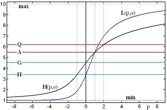
The two lines trace the Hölder path (black) and the Lehmer path (blue). The horizontal lines indicate, for the same set a, the minimum (lowermost), the harmonic mean H, the geometric mean G, the arithmetic mean A, the quadratic mean Q and the maximum (uppermost).
3. Abstract definitions of means and averages
The terms mean value and average value are often used as synonyms but they are actually two quite different concepts.
The three examples which follow should help to clarify the difference.
Example 1: One can hardly object to the physical concept of an average force on a body, while there is something amiss in the hypothetical term mean force. The problem is that forces are 3D vectors and they can cancel even when non of them is zero. The idea of several non-zero entities averaging to zero is acceptable, but it conflicts with the intuitive notion of a mean value.
Example 2: A finite subset of complex numbers may have an average compatible with formula (1) but it is not a mean for, due to the lack of definition of a minimum (or a maximum) of a set of complex numbers, there is no way to check the condition (m3). Actually, this applies also to the preceding case and, vice versa, the objection of the previous example holds also for this one.
Example 3: Consider the quadratic mean of Eq.(4) with p=2, and apply it to a finite set of real numbers, admitting also negative values. The formula is then still legitimate and amounts to an average known as the root-mean-square. But it is not a mean since, for example, the rms of {1,-2} is positive and therefore, again, does not satisfy the condition (m3).
From these examples it is evident that the difference lies in the condition (m3) which needs to be satisfied by means but not by averages. We will now try and define the terms mean and average for as wide categories of sets as possible, exploiting the insight about (m3) for a formal distinction between the them.
Definition: Let e ≡ {ek; k = 1, 2, ..., n} be a non-empty, finite subset of a domain set S which satisfies some conditions to be defined later. Denoting as E the set of all such subsets, we call a mean any mapping ME → S satisfying the following conditions:
- M1) Symmetry: M(P(e)) = M(e).
- M2) Linear scaling: M(ce) = c M(e), where ce = {cek; k = 1, 2, ..., n} and c is any element of an algebraic field F.
- M3) Bounds: min(e) ≤ M(e) ≤ max(e).
The condition (M1) does not impose any limitation on the set S. Condition (M2) requires that the product ce, where c is any element of F (such as a real number) and e is any element of S, must exist and be an element of S. The simplest (though not unique) way to satisfy this requirement is for S to be a linear vector space over F. Examples of such sets include those of real and complex numbers, n-D vectors, matrices of a given size NxM, tensors, functions of real or complex variable, etc.
Finally, the condition (M3) makes sense only when the set S is totally ordered since only then the minimum and maximum elements are uniquely defined. Of the above listed sets, only that of real numbers has this property, which is the reason why means are usually defined straightaway just for the set of real numbers R or for some of its subsets.
Average: To define an average, it is now sufficient to drop condition (M3) and the restrictions on the set S which it implies.
This makes means a special case of averages - every mean is an average, but not vice versa. It also implies that every statement one can make about averages applies also to means, but not the other way round. For this reason, we will from now on use the term average more often than mean, reserving the latter for situations in which the condition (M3) and the strong ordering of S are essential.
***** Imperfect averages and means: One can define another entity by dropping the condition (M2). Thus an imperfect average has to satisfy only (M1), and an imperfect mean must satisfy (M1) and (M3). We will encounter the latter category in Section 7 when discussing the ways of introducing new averages and means.
***** Weighed averages and means: An often used term is that of a weighed average which is a concatenation of two mappings:
Given an ordered n-tuple w ≡ {wk; k=1,2,...,n} of elements of the field F such that Σkwk = 1 (the weights), and any ordered n-tuple e ≡ {ek} of the elements of S, form first the weighed set e' = {wkek} ≡ W(w;e) and then evaluate its average (or mean) M(e').
Considering w as fixed and e as variable, the combined mapping Mw(e) = M(W(w;e)) maps n-tuples of S onto S but, since it does not satisfy condition (M1), it is not really an average at all. Rather than weighed average, it should be called average of weighed n-tuples. Moreover, since the weights are defined a-priori, the number n of elements in e is pre-defined as well. These two facts indicate that weighed averages are something quite different from the averages and means we are discussing here.
4. Basic properties of averages and means
The most important properties of averages are those imposed by the definition, namely (M1), (M2) and, for means, (M3). Beyond these, perhaps the most striking property can be loosely expressed by saying that an average of averages is again an average and, similarly, a mean of means is again a mean. Let us now make these concepts a bit more rigorous:
***** Composition theorem: Considering that any average of a given finite subset e ≡ {ek; k = 1, 2, ..., n} of the elements of S is again an element of S, a set of such averages {Mi(e); i = 1, 2, ..., m} may be used as an argument of an average M0.
The combined mapping
(6) M(e) = M0({Mi(e)})
then satisfies conditions (M1), (M2) and therefore is also an average. When M0 and all the Mi are means, M satisfies also the condition (M3) and therefore is also a mean.
Example: the arithmetic mean of the arithmetic and harmonic means is again a mean
For averages, this can be generalized as follows:
***** Weighed composition of averages: Given an average M0 on a set S, an m-tuple {Mi; i = 1, 2, ..., m} of averages on S, and a corresponding m-tuple {wi} of elements of F, the following composite mapping is also an average on S:
(7) M(e) = M0({wiMi(e)})
Unlike weighed averages, the weighed composition of averages is compatible with (M1) because the weighting coefficients are not applied directly to the elements of e but to the means which are themselves invariant under permutations of e.
Extending the last theorem to means requires the introduction of the following property:
***** Monotonous averages and means: An average (or a mean) M on a totally ordered set S is monotonous if it satisfies the following condition: Let e, e' be two n-tuples of elements of S such that ek ≤ e'k for every k =1,2,...,n. Then M(e) ≤ M(e').
Considering the invariance under permutations of e, this is equivalent to saying that a monotonous average or mean M(e) does not decrease when any of the elements of e increases. One can sharpen this definition by requiring M(e) to actually increase whenever an element of e increases, and call such averages strictly monotonous.
Of the particular means we have discussed so far, all are monotonous, except the Lehmer mean for some values of p. Most of the monotonous means are also strictly monotonous, except the minimum and maximum, the median, and the robust means which need not necessarily change when one of the elements of e changes.
***** Weighed composition of means: Let M0 be a monotonous average on a totally ordered set S, {Mi(e); i = 1, 2, ..., m} an m-tuple of means on S, and {wi} a corresponding m-tuple of elements of F such that M0({wi}) = 1. Then the composite mapping
(8) M(e) = M0({wiMi(e)})
is a mean on S.
***** Continuous averages and means: When S, apart from any other required properties, is also a topology, the mapping M(e) may, but need not, be continuous with respect to any one of the elements of e (due to the permutation symmetry it does not matter which one we pick). When it is continuous, we say that the average (or mean) is continuous.
***** Regular averages and means: We will say that an average, or a mean, is regular when it is both monotonous and continuous. Similarly, it is strictly regular when it is both strictly monotonous and continuous.
Of the particular means discussed so far, all are continuous. With the exception of the Lehmer mean they are all regular, but only the Hölder means (with all their special cases) in R+ are strictly regular.
***** Simple averages and means: Given an n-tuple e of the elements of S and any other element x of the same set, we will denote as {e,x} the subset of (n+1) elements containing all the members of e, plus the element x. Given an average (or a mean) M on S and an n-tuple e, we can now ask whether there is an element x of S such that
(9) M({e,x}) = M(e)
The solutions of equation (9) depend both upon the particular mapping M and upon the set e. Given an e, the number of such solutions may be anything, including zero and infinity. When (9) has exactly one solution for every subset e whose elements are all different, we say that the average (or mean) M is simple. When this holds for any e, regardless of whether its elements are all different or not, we say that M is totally simple.
***** Stable averages and means: An average (or mean) M on a set S is said to be stable if, for every finite subset of S, the value M(e) is a solution of equation (9):
(10) M({e,M(e)}) = M(e).
Note: To be stable, an average must admit at least one solution of equation (9), namely x = M(e). It does not need to be simple, however, since there might exist also other solutions. Thus, for example, the min and the max are stable but not simple since, for these means, any x which lies between the minimum and the maximum of e is a solution of (9).
***** Coherent averages and means: Given m different n-tuples ek, k = 1,2,...,m, of the elements of S, let e' be their union. An average (or a mean) M on S is said to be coherent if, for any choice of the n-tuples ek,
(11) M(e') = M({M(e1),M(e2),...,M(em)}).
5. Computability of means and averages
Consider the evaluation of the elementary means (max or min). It is numerically extremely efficient since it requires only one fast floating point operation for each element of a. Similarly, the arithmetic mean (or average) is very efficient since it takes just one addition per element, plus a single division at the end. No other mean matches this degree of efficiency.
In general, efficiency could be defined as the inverse of the number of clock cycles which an ideal processor needs in order to handle a single element of a. In practice, however, efficiency may be difficult to evaluate since the number of clock cycles required to execute floating point operations differs from processor to processor. As a rough estimate, one can just count how many simple arithmetic operations (+,-,*,/) per element of a are needed.
The arithmetic mean has also another advantage. There are many practical situations when a data evaluation unit is presented sequentially with a large number of data values and required to return their average (or mean) without any permanent storage of the individual items. This is typical of all data accumulation (data averaging) devices. In such cases one obtains the desired result by means of the following recipe:
1) First, zero two 'registers', namely an accumulator A and a counter N.
2) Every time a new datum becomes available, add it to A and increment N by 1.
3) At the end, the mean value is obtained by dividing the final value of A by that of N.
The point is that, apart of a few registers, one does not need any large hardware memory buffer to store the individual data values.
We will call thrifty any average or mean for which there exists an algorithm having this property.
To be thrifty used to be a great advantage some 40 years ago when 1 Kbyte of memory used to carry a price tag in excess of $1000. It is much less important today when, in inflation-adjusted terms, the memory cost is about 9 orders of magnitude less. Nevertheless, there are situations (like hard-wired or FPGA designs) where the memory storage needed to hold all the individual data values might take up too many hardware resources.
Among the classical means mentioned above, most are thrifty (the only exceptions are the median and the robust means). The efficiency varies a lot, though. In particular, the Hölder means with fractional p's are much less efficient than those with integer p values, due to the time it takes to compute a power with a non-integer exponent.
A still another property which has to do with computability of averages and means is an extension of the concept of coherence: Given m different subsets ek, k = 1,2,...,m, of the elements of S, let e' be their union. For many averages and means there exists a way to compute the mean of the union set e' using only the means of the partial sets ek and their sizes nk (unlike in the case of coherence, the latter are not supposed to be all the same). When such an expression exists, the average (or mean) is said to be a wrapper and the expression is its wrapper (or wrapping) formula.
6. Empirical pertinence of the basic properties of means
Means are often used in empirical situations as estimates of some quantity from a number n of measurements burdened by random measurement errors. The choice of the mean then depends upon the statistical properties of the errors as well as upon the quantity to be measured. Though this is by far not the only application of means, it is a very important one and it is quite instructive to observe the relevance of the above-defined properties in such a context.
Assume that we have carried out n measurements q = {qk; k = 1, 2, ..., n} of a quantity Q and that their chosen mean is q = M(q). In the considered context it would be somewhat puzzling if, replacing any one of the individual measurements with a higher value, the mean value q decreased. This indicates that monotonous means are favored (and the strictly monotonous ones are even better). Continuity is also appealing since its lack would imply existence of situations when an infinitesimal change of one of the measured values causes a finite jump in the value of the mean. Combined, these two facts amount to a strong preference for regular means or, better still, strictly regular ones.
Now suppose that we take another measurement and that it comes out equal to q. This we would view as a confirmation of the previous measurements (though a bit fortuitous one) and we would certainly be quite puzzled if it changed the current mean q. In other words, we expect M({q,q}) = M(q) which amounts to saying that M should be stable. There is also a preference for simple means since it may be somewhat disappointing to measure two new, mutually different values and find out that the new mean is the same no matter which one we consider.
The desirability of coherence is also easy to understand. Suppose that we divide all the measurements into two groups A and B of equal size according to some criterium unrelated to the measured quantity. For example, if the measurements are indexed chronologically, A could be the odd-indexed ones and B the even-indexed ones. Or A and B could be the measurements taken by two different persons. Now if we take the separate means for the groups A and B, respectively, and if M is coherent, then the mean of the complete set is equal to the mean of the same type of the two partial subsets. The coherence helps us to combine partial means originating from different measurements even when the individual values are no longer available. It is even better if the mean is a wrapper since in such a case partial means measured by different persons can be easily combined, using just their values and the numer of measurements done by each person, without knoing all the individual values.
If follows that in the absence of other specific indications a mean, in order to be used for empirical measurements, should be strictly regular, stable, coherent, and possibly a wrapper. Of the classical means (see Section 2), this is true only for the Hölder means (including the special cases of quadratic, arithmetic, geometric and harmonic means) and thus explains their popularity and importance.
Table 1. Properties of the classical means
Thrifty means show in parentheses the number of needed arithmetic registers (excluding the counter).
Efficiency is indicated by the required number of various arithmetic operations per item.
For proofs, click the name of the mean.
| Mean | Domain | Monot. | Cont. | Regular | Simple | Stable | Coherent | Wrapper | Thrifty | Efficiency |
| Minimum |
R | Yes | Yes | Yes | No | Yes | Yes | Yes | Yes (1) | 1 < |
| Maximum |
R | Yes | Yes | Yes | No | Yes | Yes | Yes | Yes (1) | 1 < |
| Median |
R | Yes | Yes | Yes | No | Yes | No | No | No | O(n ln(n)) < |
| Arithmetic |
R | Strict | Yes | Strict | Yes | Yes | Yes | Yes | Yes (1) | 1+ |
| Robust |
R | Yes | Yes | Yes | No | No | No | No | No | O(n ln(n)) < |
| Geometric |
R+ | Strict | Yes | Strict | Yes | Yes | Yes | Yes | Yes (1) | 1* |
| Harmonic | R+ |
Strict | Yes | Strict | Yes | Yes | Yes | Yes | Yes (1) | 1i, 1+ |
| Quadratic | R+ |
Strict | Yes | Strict | Yes | Yes | Yes | Yes | Yes (1) | 1*, 1+ |
| Hölder | R+ |
Strict | Yes | Strict | Yes | Yes | Yes | Yes | Yes (1) | 1^, 1+ |
| Lehmer | R+ |
No | Yes | No | Yes | Yes | No | No | Yes (2) | 1^, 1*, 2+ |
Inequalities involving means and averages
There are many important inequalities applicable to the various classical averages and means which hold for any choice of the argument set a. Here we will mention only the most important ones, all well illustrated by Figure 1. The author, in fact, finds graphical tools like Figure 1 very useful for the discovery, comprehension and memorization of many inequalities. Any tendency one detects in such a graph, especially if checked for persistence with various argument sets a, usually turns out to be universally true (although a final rigorous proof is still required).
Note: In the inequalities appearing in this Section, the equality sign applies if and only if all the elements of a have the same value.
***** Hölder mean inequality.
As an example, consider that the Hölder path H(p,a) defined by Eq.(4).
Since it is for any a a monotonously increasing, continuous function of p, we have
(12) When p < q then H(p,a) ≤ H(q,a).
This is probably the most important of all inequalities on means and it turns up in many contexts, some of which apparently quite unrelated to the present topic. It should not be confused with the more commonly cited Hölder inequality which is something else.
A direct consequence of the fact that dH(p,a)/dp ≥ 0 is the following inequality, equivalent to (12),
which holds for any set of n positive real numbers zk:
(13) Σ[zkln(zk)] > (Σzk) ln[(Σzk)/n] or, using the arithmetic mean, A({zkln(zk)}) > A(z) ln(A(z)).
Considering the special means (harmonic H, geometric G, arithmetic A, and quadratic Q) along the Hölder path,
inequality (12) leads directly to:
(14) min(a) ≤ H(a) ≤ G(a) ≤ A(a) ≤ Q(a) ≤ max(a).
These inequalities, combined with others such as (13), produce a bewildering number of derived inequalities applicable to totally generic sets of positive real numbers, many of which are very useful in a broad range of practical applications.
***** Lehmer inequality.
Since the Lehmer path L(p,a), defined by Eq.(5) is also a continuous, increasing function of p, we have:
(15) When p < q then L(p,a) ≤ L(q,a).
One also notices that
(16a) When p ≥ 1, L(p,a) ≥ H(p,a)
(16b) When p ≤ 1, L(p,a) ≤ H(p,a)
Construction of new means
We have already seen how the composition theorems can be used to derive new averages or means starting from ones which had been defined previously. We will now discuss two more approaches to defining new means. The first one is purely mathematical and, like the composition means, relies on pre-defined means. The other one is more application-oriented and looks for inspiration in geometry, physics and other extra-mathematical areas.
***** Generalized means
Let f:D→D' be a continuous and strictly monotonous function which maps a suitable real-numbers domain D onto an image domain D' and let g:D'→D be its inverse, so that g(f(x)). Suppose further that D' is closed under addition (i.e., when a,b belong to D' then so does a+b). Then the following expression satisfies conditions (m1) and (m3):
(17) 
The Hölder means, for example, follow from (1) by setting f(x) = xp.
Other important special case are:
Exponential mean, defined on the whole of R, obtained by setting f(x) = exp(x), g(x) = ln(x).
Inverse exponential mean, also defined on R, obtained by setting f(x) = exp(-x), g(x) = -ln(x).
Logarithmic mean, defined on R+, obtained by setting f(x) = ln(x), g(x) = exp(x).
However, the logarithmic mean is identical to the geometric mean (equation 2) and thus does not represent anything new, while the exponential and inverse exponential means do not satisfy condition (m2) and thus are likely to be of less use in practical applications, unless the averaged quantities are dimensionless. They are examples of the imperfect means defined above.
However, there is a simple way of removing the imperfection. When M(a) is any selected mean, then the following formula defines a new, normalized generalized mean which satisfies all three conditions:
(18) 
Further generalization is possible using two means (not necessarily different ones) M(a) and M'(a), and setting
(19) F(a) = M(a) g(M'({f(ak/M(a)})).
Expression (18) is in fact a special case of (19) with M'(a) being the arithmetic mean.
Using equations (6), (8) and (19) in various combinations and in an iterative way, one can define an absolutely bewildering number of distinct composite and generalized means starting from a few pre-defined ones.
***** Application-defined means
In practice, means arise in various contexts such as statistics, statistical physics, geometry, numeric approximations of functions, and many more. To illustrate the process, let us see just one example taken from geometry.
Consider an n-dimensional ellipsoid with semi-axes {ak}, k=1,2,...,n. In many applications one is interested in either the "volume" or the "surface" of such an ellipsoid. The numeric expressions for these quantities may be more or less difficult to derive. In this example, the volume presents no problem, while the surface involves transcendental functions and presents considerable computational problems even for n = 2. In any case, however, one can introduce the concept of an "equivalent sphere", i.e., an n-dimensional sphere which has either the same volume or the same surface.
It can be easily shown that the radii of such equivalent spheres are means of the semi-axes {ak}. Naturally, volume and surface lead to different kinds of means. The equivalent volume radius turns out to be the geometric one G(a), while for surface there does not exist any generic formula. However, the definition holds and is perfectly valid; we can denote the radius of the sphere with equivalent surface E({ak}) and call E(a) the elliptic mean of a.
Whether we know how to compute the elliptic mean has nothing to do with its legitimacy; our inability to do so just indicates that it is probably neither efficient nor thrifty (and not a wrapper). What one is strongly tempted to do in these cases is to approximate the new mean arising from an "application" by means of other means which are more conventional and easier to compute. The example of ellipse perimeter (n=2) shows that even that can be a complex task.
|