1. Introduction

In the realm of real functions of real variable, convex functions constitute a conspicuous body both because they are frequently encountered in practical applications, and because they satisfy a number of useful inequalities and theorems. The most important of the inequalities is of course the defining one which states that a real function f(x) defined on a real-numbers interval X = [a,b] is convex if, for any three elements x₁, x, x₂ of X such that x₁ ≤ x ≤ x₂,

(1)   f(x) ≤ f(x₁)*[(x₂ - x)/(x₂-x₁)] + f(x₂)*[(x - x₁)/(x₂-x₁)]

Graphically, as shown in Figure 1A, this means that the point {x,f(x)} never falls above the straight line segment connecting the points {x₁,f(x₁)} and {x₂,f(x₂)}.

The definition (1) can be easily extended to any kind of real-numbers interval, though in this article we will be only concerned with the closed and finite ones. Convex functions satisfy a number of theorems, the most important of which are:

Theorem 1) f(x) is continuous at all inner points of X.
Theorem 2) f(x) has in X at most one local minimum which, if it exists, is also its absolute minimum in X.
Theorem 3) When f(x) has a second derivative at a point x of X, its value is non-negative.

Other theorems can be found in references [1] and scattered over a vast literature. Notice that while convexity implies continuity, it does not imply the existence of first or higher derivatives, nor does it imply monotonicity (see the examples in Figure 1B).

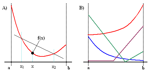
Figure 1. Illustration of basic concepts

A) Definition of a convex function. B) Examples of convex functions.
 

2. The theorem

Let X = [a,b] be a finite, closed real numbers interval and let f(x) be a finite-valued real function defined everywhere on X.
Divide the interval [a,b] into K equally wide sub-interval by means of K+1 points {x_k, k = 0,1,...,K},
where x₀ = a, x_K = b, and x_k - x_k-1 = (b-a)/K. Define further the quantity

(2)   A(K;f) = Σ_k=0:Kf(x_k)/(K+1).

The theorem we want to prove can be now stated as follows:

When f(x) is convex then, for any K ≥ 1,
(3)   A(K+1;f) ≤ A(K;f).

Before facing the proof, let us spend a few words about the meaning of inequality (3):
A(K;f) is simply the arithmetic average of the values {f(x_k)}. Under the specified conditions, the integral J of f(x) over X exists and, for large K, can be approximated by (b-a)A(K;f) and the sequence A(K;f) converges to J/(b-a). The theorem implies that when f(x) is convex, the sequence A(K;f) not only converges to a limit, but it does so in a monotonous way.

3. The proof

First, let g(x) = f(x_c-(x-x_c)), with x_c = (a+b)/2 being the central point of the interval X. Then g(x) is a horizontal reflection of the function f(x) about x_c and s(x) = [f(x) + g(x)]/2 is symmetric about x_c (see Figure 2A for an illustration).

It is evident that the symmetrized function s(x) satisfies the pre-requisites of the theorem and that

(4)   A(K;f) = A(K;s).

The latter identity follows from the fact that the points {f(x_k)} are also distributed symmetrically about x_c.
Consequently, for any k, f(x_k)+f(x_K-k) = f(x_k)+g(x_k) = 2.s(x_k) = s(x_k) + s(x_K-k).

This entitles us, without any loss of generality, to limit the discussion to convex functions s(x) symmetric with respect to the center x_c of X. In other words, if inequality (3) holds for any finite, symmetric convex function s(x) than it holds also for any finite and convex function f(x), regardless of whether it is symmetric or not. Notice that all convex functions which are symmetric on X necessarily have at x_c a unique local minimum which is also their global minimum in X.

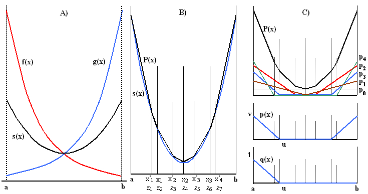
Figure 2. Illustrations for the proof for K = 4 (see the text for details)

Consider now the following sets of ordinates (for an illustrative example, see Fig.2B):
(5a)   {x_i, i = 0,1,...,K}, where x_i = a + i(b-a)/K, appearing in A(K;s) and
(5b)   {x'_j, j = 0,1,...,K+1}, where x'_j = a + j(b-a)/(K+1), appearing in A(K+1;s).

For any K, the two sets have exactly two elements in common, namely x₀ = x'₀ = a and x_K = x'_K+1 = b. The nonius-like behaviour associated with the fact that we consider division of X into K and K+1 intervals (rather than some generic K and K') is essential in this step and makes the inner points of the two grids intercalate in a regular way. The union of the two sets therefore contains exactly 2K+1 distinct ordinates
(6)   {z_i, i = 0,1,...,2K} such that for even i, z_i = x_i/2 and for odd i, z_i = x'_(i+1)/2.
Notice that z₀ = a, z_K = x_c, and z_2K = b.

Consider now the symmetric convex polygon P(x) formed by the points [z_i,f(z_i)] as shown in Figure 2B. Clearly

(7)   A(K;s) = A(K;P) and A(K+1;s) = A(K+1;P).

This, together with Eq.(4), indicates that if we prove the validity of inequality (3) for the symmetric convex polygon P(x), its validity for any convex function f(x) will be proved.

This reduction process can be extended further exploiting the nearly obvious fact (elementary algebra is sufficient to verify it) that when f(x) and g(x) both satisfy the assumptions of the theorem and v, w are any non-negative real numbers, then the combination v.f(x)+w.g(x) also satisfies the requisites (in particular, it is finite and convex) and A(K,v.f+w.g) = v.A(K,f) + w.A(K,g). We will refer to this property as the superposition Lemma.

In particular, the polygon P₀(x) = P(x) can be expressed as a sum of K+1 special symmetric convex polygons p_k(x), such as those shown in Figure 2C. These are constructed as follows:

• Set p₀(x) = P₀(z_K) and P₁(x) = P₀(x) - p₀(x). The constant function p₀(x) is the first of our special polygons (black).
  Since P₀(z_K) is the minimum of P₀(x) in X, P₁(x) is a symmetric convex polygon whose value at the central point is zero.
• Now define the second of our special polygons (brown), p₁(x) as being composed of two linear segments, one of which passes through the points [z_K-1,P₁(z_K-1)] and [z_K,0] and the other one is positioned symmetrically. Due to the convexity of P₁(x), the difference P₂(x) = P₁(x) - p₁(x) is a symmetric convex polygon which is zero at the points z_K-1, z_K and z_K+1.
• The subsequent special symmetric convex polygons p_k(x), k = 2 (red), 3 (blue), ..., are all composed of three linear segments: two symmetrically placed sloping ones and a central section where their value is zero. More specifically, p_k(x) is zero at points z_K-k+1 through z_K+k-1 and its left linear segment passes through the points [z_K-k,P_k(z_K-k)] and [z_K-k+1,0]. The residual polygons P_k(x) are defined by the recursive formula P_k+1(x) = P_k(x) - p_k(x) and are all symmetric and convex.
• The reduction process clearly terminates with p_K(x) because the residual polygon P_K+1(x) is everywhere zero.
  Consequently, we have P(x) = Σ_k=0:K p_k(x).

According to the superposition Lemma, it is now sufficient to prove that each of the special polygons p_k(x) satisfies inequality (3). Since this is obvious for k = 0 (any mean of a constant is always equal to the constant itself), we need to show that it holds for any k ≥ 1. One can carry the reduction one step further by taking any symmetric special convex polygon p_k(x) such as the one in Figure 2C, middle, and splitting it into two components, one of which is the function q_k(x) shown in Figure 2C, bottom, and the other is its symmetric reflection. In virtue of the superposition, if inequality (3) holds for q_k(x), it holds also for its symmetric reflection, and therefore also for p_k(x) which is the sum of the two, multiplied by some non-negative constant.

The proof of the validity of inequality (3) for functions of the form of q_k(x) will be carried out explicitely. We have

   q(x) = (u-x)/(u-a) = 1-(x-a)/(u-a) for x ≤ u and q(x) = 0 for x ≥ u, where u coincides with one of the points z_k, k = 1, 2, ..., K.

To evaluate A(K;q) and A(K+1;q) we will consider two cases:

I) Let k = 2m be even with 1 ≤ m ≤ K/2. In this case u = z_k = x_m and we have

(8a)   

(8b)   

In this case, therefore, A(K+1;q) = A(K;q), which is compatible with (3).

II) Now let k = 2m-1 be odd, again with 1 ≤ m ≤ (K+1)/2. Then u = z_k = x'_m and we obtain

(9a)   

(9b)   

Since m < K+1, we see that in this case A(K+1;q) < A(K;q) and inequality (3) is again satisfied.

This completes the proof.

4. Final remarks

The theorem proved above may appear intuitive and therefore little exciting, and yet its proof is relatively complex, showing that inequality (3) is cutting it very close in some cases. The following considerations illustrate this point and, in a way, explain why the inequality is not trivial.

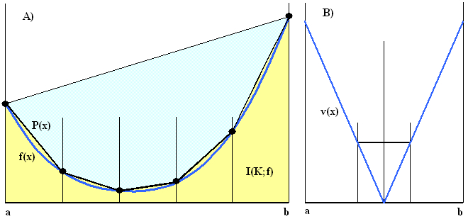
Figure 3. Definite integral approximations (see text for explanations)

Consider a bounded convex function f(x) over an interval X = [a,b] such as the one shown in Figure 3A. If the interval is divided evenly into K parts then the integral I(f) of f(x) over X can be approximated by the area I(K;f)) of the K trapezoids shown in yellow. Elementary geometry gives

(10)   I(K;f) = (d/K)[Σ_i=0:Kf(x_i) - (f(x₀)+f(x_K))/2], where d = b-a and d/K is the width of the trapezoids.

Which, of course, is just one of the Simpson numerical integration rules.

Notice that, while the values I(K;f) are all greater than their limit I(f), their sequence is NOT necessarily monotonous. An example is shown in Figure 3B; for the v-shaped convex polygonal function v(x) we have I(K;v) = I(f) for any even K, but I(K;v) > I(f) for any odd K. In particular, I(3,v) > I(2,v). According to the theorem, however, the arithmetic averages A(K;f), as well as A(K;v), are guaranteed to form a monotonous, non-increasing sequence.

Substituting Σ_i=0:Kf(x_i) with (K+1)A(K;f), one obtains

(11)   I(K;f) = d (1+1/K) A(K;f) - I(1,f)/K, where I(1,f) = d (f(x₀)+f(x_K))/2 embodies the interval edge effect.

For positive convex functions f(x) the non-monotonous behaviour of I(K;f), when present, is therefore due essentially to the edge effects. The first term is in fact a product of two decreasing factors (1+1/K) and A(K;f), while the edge-effects term -I(1,f)/K is increasing and may sometimes prevail. When f(x) is convex but negative, the situation is a bit more complex since A(K;f) is negative and decreasing (which makes it increasing in absolute value) while (1+1/K) is a decreasing positive factor. This makes the behavior of their product somewhat unpredictable.

In any case, combining equation (11) with inequality (3), one obtains an interesting general inequality for I(K;f) which, among other things, places a bound upon the I(K;f) non-monotonicity:

(12)   I(K+1;f) - I(K;f) ≤ [I(1,f) - I(K;f)]/(K+1)²

Notice that the quantity [I(1,f) - I(K;f)] is graphically represented by the light blue area in Figure 3A and converges rapidly to the area enclosed between the straight line connecting the end points of f(x) and the function f(x) itself. The v-shaped polygon of Figure 3B constitutes an example where, for even values of K, the equality in (12) is actually attained.

Let us now return to inequality (3) and see some of its properties and implications. First of all, it is clear that it implies

(13)   A(K;f) ≤ A(K';f) whenever K' < K.

Another trivial extension regards concave functions. When f(x) is concave then -f(x) is convex and must satisfy inequalities (3) and (13). This implies that for concave functions the ≤ relation sign is simply replaced by the ≥ sign.

The question now is when does the inequality reduce to equality. One obvious case is when f(x) is constant since then all the f(x_i) are the same and all their arithmetic averages equal the common value. From the proof, however, we have seen that for some specially constructed convex polygons p(x) and some particular K values the equality A(K+1;p) = A(K;p) can arise. For K > 2 there exist more than one such polygon and therefore the equality occurs also for any of their linear combinations. On the other hand, a closer inspection reveals that in such cases the equality happens only for some values of K, never for every K. The situation can be summed up as follows:

When f(x) is a constant, inequality (3) becomes equality. Otherwise, the inequality is always sharp, unless f(x) is a convex polygon, in which case it might in some special cases become an equality for special values of K (in this article, no detailed analysis of the special cases is carried out).

Another question is whether the implication of the theorem could be inverted, i.e., whether the validity of (3) for any K implicates that f(x) is convex. This seems highly unlikely. One can imagine a function f(x) which is convex everywhere in the interval X except in a narrow sub-interval C. Then, as far as inequality (3) is concerned, the regions where f(x) is convex could always outweigh the opposite behavior in the interval C.

5. Extensions

As a final exercise, let us try and extend inequality (3) to means other than the arithmetic one [reference 2]. Since a positive convex function f(x) remains convex when elevated to a power p ≥ 1, inequality (3) can be applied to f^p(x). Both sides being positive, we can elevate them to the power 1/p without violating the inequality. Consequently, given a finite interval X = [a,b], a function f(x) which is in X positive and convex, and any real p ≥ 1, we have H_p(K+1;f) ≤ H_p(K;f), where H_p(K;f) denotes the Hölder mean with parameter p of the values {f(x_i); i = 0,1,2,...,K; x_i = a+i(b-a)/K}.

For positive convex f(x) and p ≤ -1, the function f^p(x) is concave. Applying to it the concave version of the theorem and elevating both sides to 1/p (attention: the exponent being negative, this operation reverses the inequality!) we obtain the same result. Hence, combining the two insights, we conclude that

(14)   for positive convex f(x) and any real p such that |p| ≥ 1, we have H_p(K+1;f) ≤ H_p(K;f).

The most important special cases of (14) are the quadratic mean, obtained for p = 2, and the harmonic mean (p = -1).

An altogether analogous reasoning can be carried out for positive concave functions and Hölder means with -1 ≤ p ≤ 1.
This leads to the realization that

(15)   for positive concave f(x) and any real p such that |p| ≤ 1, we have H_p(K+1;f) ≥ H_p(K;f).

Since limit transitions do not reverse inequalities, this applies also to the geometric mean, obtained for p = 0.

The generalized inequalities (14) and (15) also stress the special standing of the arithmetic and harmonic means which are the only ones to which both of them are applicable.