|
References
Hebel-Slichter-Redfield field-cycling NMR experiment
This experiment was designed [11,12] to measure longitudinal relaxation rate R1 (inverse of the relaxation time T1 ) of nuclides in both normal and superconducting metals at various applied magnetic fields B (including zero field). Using current terminology, we recognize in it an almost standard [27] Fast Field-Cycling NMR Dispersion Relaxometer (FFC-NMRD). The original instrument operated in continuous way (CW) as follows (Figure 1):
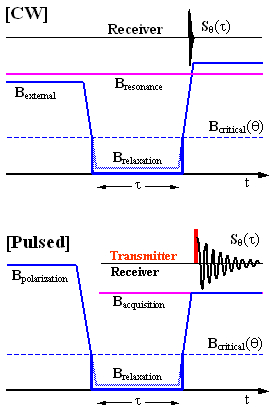
Figure 1. Timing diagram
of the Hebel-Slichter-Redfield experiment
The sample's nuclides are first polarized in a relatively large applied magnetic field (the thin blue line). This is then switched to the desired Brelaxation (or just Br ) value at which it is left to relax for a variable time τ. The field is then switched to a value which is somewhat higher than the resonance field corresponding to the continuously applied radiofrequency. As the magnetic field flies across the resonance condition one detects a brief, ringing signal S(τ) whose intensity, of course, depends upon τ and also upon the relaxation field value and the absolute sample temperature θ.
Plotting S(τ) as a function of τ, one obtains the relaxation curve for longitudinal magnetization which passes from its equilibrium value in the polarization field to that in the relaxation field. In most metals, this curve is mono-exponential and its decay rate coefficient is the measured value of R1(θ,Br).
The modern, pulsed version of the experiment is conceptually similar, but the transmitter and the receiver are both gated, the polarization field can be much higher (there is no interference with nuclear magnetization when the field is switched down) and the signal is acquired at a constant field close to resonance (or even on resonance), giving a well-behaved free induction decay (FID). The consequent gain in sensitivity and precision is obvious.
While this experimental setup is quite universal, in the case of metals the explanation really applies only to non-superconducting samples. Due to the Meissner effect [3,4], the internal magnetic field in a superconductor is rigorously zero even in the presence of an external field (no matter whether static or dynamic). Consequently, whenever the applied field drops below a critical field level, the effective internal field perceived by the sample's nuclides becomes abruptly zero, as indicated by the thick blue line in Figure 1.
Consequently, the only relaxation rate one can measure in a superconductor is that at zero magnetic field.
A few facts about relaxation in normal metals
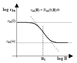
Figure 2. NMRD profile of a normal metal
Dispersion profiles are best plotted on a log-log scale, as indicated by the labels of the axes. Following usual conventions, however, specific values are indicated without the log in front.
We want to avoid theory here but it is useful to recall at least the phenomenological aspects of NMR relaxation in normal metals which were known [9,10,11] already in 1957, the year when the Hebel-Slichter effect was discovered.
First of all, the longitudinal relaxation rate R1n(θ,B) in a normal metal is typically proportional to the absolute temperature θ and can be normalized by plotting the ratio r1n = R1n/θ as a function of the applied magnetic field B. The normalized NMR dispersion curve looks typically as shown in Figure 2. There is a plateau at both low and high fields and a dispersion region around some value Bd which depends upon the particular metal. According to early theoretical models [10,12], the ratio r1n(0)/r1n(∞) should be equal to 2, but actual experimental values often deviate considerably.
In non-superconducting aluminum, for example, the center of the dispersion region is at Bd = 1.5 mT, the temperature coefficients are r1n(0) = 2.2 s-1K-1 and r1n(∞) = 0.6 s-1K-1, their ratio is 3.3, and the maximum log-log slope at the inflex point is -0.6 (the oblique dotted line).
In any case, it is relatively easy to measure NMRD profiles of powdered metal samples, determine their longitudinal-relaxation dispersion parameters, and use the latter to extrapolate the R1n(θ,B) values to any temperature θ and any magnetic field B.
A few facts about superconducting metals
Some metals become superconductors when their absolute temperature θ is lower than a critical value θc and the external magnetic field B does not exceed some critical value Bc(θ) which decreases with increasing temperature and becomes zero at θc. In a [B,θ] diagram (Figure 3 on the right), the boundary of the region where a metal is in a superconducting state can be approximated quite well by a formula containing just two parameters, the θc and Bc = Bc(0).
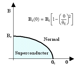
Figure 3. State diagram of a superconductor
Figure 3 is reminiscent of a phase diagram of a substance, especially when one considers that electric and magnetic field intensities are legitimate thermodynamic state variables. The question is what is the substance, and it is not difficult to guess that it must be the electron gas of the delocalized metal electrons. Superconductivity therefore implies something akin to a phase-transition. That much became clear relatively soon after its discovery by Heike Kamerlingh Onnes [1,2] in 1910, but the nature of the phenomenon remained unclear for nearly half a century. The subsequent history up to - and including - the BCS theory [16-21] born in 1957 is well described in Wikipedia, so we can skip it here. Suffice it to say that the BCS theory is based on a microscopic phenomenon - the formation of quasi-persistent and quasi-localized electron pairs (Cooper pairs). Since the spins of the two electrons in such a pair are anti-parallel, these pseudo-particles have zero total spin and thus behave as doubly charged bosons - something totally different from normal electrons which, being fermions, must obey the rigors of Pauli's exclusion principle. I am of course oversimplifying a complex phenomenon which involves interactions of electrons with phonons and second quantization of the electron field, but the general idea is just that.
Not all metals have a superconducting region and not all superconductors have such a neat diagram. But let us consider a well-behaved metal like aluminum (Bc=9.84 mT, θc=1.172 °K) and see what its superconductivity diagram implies when it comes to the Hebel-Slichter-Redfield experimental setup of Fig.1. When the field is switched from a high value (well above Bc ) to near zero, or vice versa, it at some point crosses the critical value Bc(θ) indicated in Figure 1 by the dotted blue horizontal line. When changing the sample temperature θ (but staying below θc), the Bc(θ) moves vertically up or down. It is evident from the timing diagram, however, that this does not particularly affect the experiment. So, in principle, R1 values can be measured in the superconductive region at any absolute temperature between 0 and θc.
For completeness, let us say that the dynamics of the normal-to-superconducting transition is very fast and does not interfere with the experiment (at least, nobody has ever complained about it and I don't know whether it has been ever measured).
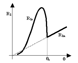
Figure 4. Experimental Hebel-Slichter peak
The indices s and n refer to the superconducting and normal state, respectively.
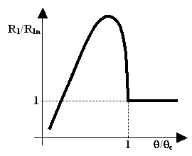
Figure 5. Normalized Hebel-Slichter effect
Hebel-Slichter effect
Now we know how to measure the longitudinal relaxation rate R1 of a metal's nuclides at any absolute temperature θ and at relaxation field Br = 0 (the latter value is imposed by the fact that in the superconducting state we are not free to set it at will). We even know what to expect of the curve R1(θ) = R1(θ,0) in the normal state (a linear dependence). So what if we now measure R1(θ) at all temperature values, covering also the superconducting region?
The experimental result [11,12,13] is shown schematically in Figure 4. Just below the critical temperature, the relaxation rate abruptly increases above the expected 'normal' value. In the superconducting state, the value of R1s(θ) reaches its maximum at absolute temperature which is about 80% of θc and then, at temperatures below about 10% of θc, drops even below the extrapolated 'normal' value R1s(θ) indicated by the dotted line. This R1s temperature profile is known as the Hebel-Slichter peak.
To account for and, to some extent, eliminate the 'normal' contributions to longitudinal relaxation, it is useful to normalize R1(θ) dividing it by R1n(θ) (either measured or extrapolated). When the absolute temperature is also normalized dividing it by θc, one obtains a graph like that shown in Figure 5, where the deviation from the normal value of 1 is due entirely to the dynamics of the Cooper pairs. A little bit below θ = θc the peak reaches a height of almost 3. Notice also that at low values of the ratio θ/θc, the normalized curve becomes approximately linear.
In practice, the shape of the Hebel-Slichter peak may deviate considerably from the idealized one shown in Figure 4. In some semiconductors, typically the non-metallic ones with high critical temperature, it may be even missing altogether. In all cases, however, the shape of the R1(θ) curve, especially of its normalized version, tells us a lot about the formation and dynamics of the Cooper pairs and about the phononic spectrum (lattice vibrations) of the superconducting material.
Historic notes
Longitudinal relaxation times T1 and rates R1 = 1/T1 of nuclides in metals were of interest to physicists since the early days of NMR because they, together with Knight shifts [7,8,9], throw light on the quantum states of electrons with energies lying close to the Fermi level which dominate most of every metal's properties. By late fifties, relaxation phenomena in normal metals were phenomenologically relatively well known and there were reasonably sound theoretical models to describe them.
The Hebel-Slichter experiment was carried out in 1957 at the University of Illinois by Charles P.Slichter and his pre-graduate student L.C.Hebel (sponsored by General Electric). They resorted to the field-cycling arrangement because that was (and still is) the only way to do NMR in a material which efficiently excludes any magnetic field from its interior. As they amply mention in their two key papers [11,12], they were helped a lot by Alfred Redfield [10,14,15] who was at that time a promising young NMR relaxation expert at the IBM Laboratories, respected both for his theoretical work [10] and for his experiments (he was already oriented towards variable-field NMR relaxometry). This is why I call the experiment Hebel-Slichter-Redfield's, while the effect itself is 'just' Hebel-Slichter's.
In any case, the actual experimental setup involved a specially build electromagnet with a relatively low-susceptibility yoke made of thin silicon steel plates, which permitted sufficiently fast, actively driven field switching. They polarized their powder aluminum sample in a field of about 45-50 mT and their operating frequency was 400 kHz, corresponding for 27Al to a field of about 36 mT. Aluminum was chosen because both its NMR properties and its superconductivity had been already studied by a number of investigators (including Slichter and Redfield).
The outcome of the experiments was among the key factors in discarding previous theories of superconductivity [5,12] in favor of the new BCS theory which was being concurrently developed at the same University by John Bardeen, Leon Cooper and John Schrieffer. The older theories were simply not able to explain the existence of a local extreme in the R1(θ) curve, while it was possible to slightly adapt the BCS theory to make it match the data (as acknowledged in the Hebel-Slichter papers [11,12], the two groups were in close contact).
It is interesting that the second set of experiments which cleared the way for the BCS theory regarded ultrasound attenuation [16,20]. Techniques like NMR relaxation, ultrasound absorption and dielectric relaxation are in fact closely correlated since they all reflect the same stochastic processes at atomic (or molecular) level. Combining them should be a rule.
Continuing importance
The historic aspects of the Hebel-Slicher effect, interesting as they are, should not overshadow the fact that it continues to be an important tool in the study of superconductive materials. This is particularly important for high-critical-temperature materials were the superconductivity mechanisms are still poorly understood.
It is also proper to mention here that curves remarkably similar to the Hebel-Slichter peak have been recently measured in light-scattering experiments on superfluids [26]. The parallelism, both theoretical and experimental, is so close that it is not exaggerated to speak about a generalized Hebel-Slichter effect in many systems whose quantum behavior is due to the formation (condensation) of quasi-particle pairs.
|