|
I. Definition of K-space
Suppose that a physical quantity w(r) is distributed within a region V of space. For simplicity we assume that the region V is finite and that w(r) is integrable over V (to a large extent, these conditions may be made less stringent but that is beyond the present point).
Applying Fourier transform, it is then possible to define the following complementary distribution W(k):
(1)
Here k denotes a complex vector composed of three components and dr a volume element (some prefer to write dV). The dot product k.r between r = {x,y,z } and k = {kx,ky,kz} is defined as
(2)
It is therefore evident that the distribution W(k) is defined in the linear vector space of three-dimensional complex vectors k, called the K-space, which is covariant (complementary) to our ordinary Euclidean R-space.
The two distributions w(r) and W(k) carry exactly the same information. Under a very broad range of circumstances, in fact, knowing W(k), the function w(r) can be computed from
(3)
and the solution is guaranteed to be unique.
The term K-space has been coined a long time ago in solid-state physics, where concepts like reciprocal lattice, Brillouin zones, Fermi levels and others could hardly ever been developed without it. Today, its applications span many apparently diverse fields, such as photography, X-ray scattering, electron microscopy, radio astronomy, ultrasound echography, sonar mapping, positron emission tomography, etc. Naturally, K-space has been carefully studied also by mathematicians, especially in the contexts of Bravais lattices, dual lattices, dual space groups, multi-dimensional Fourier transform, etc. Its introduction into NMR and MRI can be traced to a mention by Brown, Kincaid and Ugurbil [1], followed by a note by Ljunggren [2] and a more systematic investigation by Twieg [3]. However, considering its deep roots in physics, the concept has never been considered as particularly revolutionary by its promoters - it just filled its appropriate space in the newly developed discipline.
The notation adopted here is not unique. Many authors prefer to drop the 2π factors in the exponents in equations (1,2) in favor of angular frequency ω. In such a case, however, factors containing 2π re-appear within normalization factors in front of the integrals. For the purposes of our discussion, it is irrelevant which convention is used.
In the above formulae we have defined the 3-dimensional K-space corresponding to a 3-dimensional R-space. However, it is evident that, starting with any Euclidean space of n dimensions (n = 1, 2, 3, ...), one can extend the definition to a corresponding n-dimensional K-space. The case of n = 2 is very common in MRI in connection with techniques which pre-select a sensitive planar slice of the imaged object (likewise, it is possible to select a sensitive line and thus reduce the dimensionality to n = 1). It is well known that when spectroscopic aspects are involved, the chemical shift s can be handled as an independent dimension. The math of spectroscopic MRI therefore extends up to 4D spaces with 4D vectors {x,y,z,s}. In what follows we shall stick to normal 3D and 2D R-spaces and the corresponding K-spaces, keeping in mind that all qualitative features of what shall be discussed are valid regardless of the chosen dimensionality space.
The physical dimension of the k-vectors of any K-space is always [m-1] rather than [m] of the R-space position vectors r (m stands for meter, the unit of length). This is why K-spaces are also called reciprocal spaces.
The mathematical concept of K-space turns out to be extremely useful in a number of very diverse fields of physics. The roots of such universal usefulness can be traced to two fundamental facts:
(a) The entity w(r) can be any physical property, as long as it is possible to associate it with a distribution in space. It does not even need to be scalar - vectors, matrices and the like are all welcome. Thus in X-ray scattering w(r) stands for the electron density distribution within a material, while in NMR it is primarily the local density of the observed nuclides (we will return to this point later).
(b) In many physical experiments, the observed signals can be described in a much simpler way in the K-space than in the physical R-space. We shall see in the next Section that this applies also to the signals observed in MRI.
2. K-space and MRI signals
Let us consider first a small voxel dr located at a position r in the R-space. According to standard NMR theory, its contribution to the NMR signal (FID) is proportional to
(4)
where f is the Larmor frequency of the nuclides and the factor q(r) is primarily proportional to the local density ρ(r) of the observed nuclides. When a suitable preparatory sequence is used, however, it can be made to depend also on the relaxation times T1(r) and T2(r) and on the diffusion coefficient D(r), all intended as local properties at point r. The customary interpretation of the three factors in equation (4) is straightforward and, for the purposes of this exposition, we take it for granted. Notice, however, that we neglect chemical shift effects and consider the apparent decay rate of transversal magnetization R2* as independent of the position vector r.
When the signal component dS(t) is passed through the phase detector of an MRI scanner, the effect is to subtract from f a fixed, operator-defined reference frequency F. The difference Δf = f-F is in the audio-frequency range and is called the RF offset of the signal component, which is now described by the equation
(5)
In the absence of field gradients, one can choose F in a way to have Δf = 0 for all voxels of a sample (the on-resonance condition). However, when we apply a generic field gradient G, the Larmor frequencies of different voxels spread according to the formula
(6)
with γ being the gyromagnetic ratio expressed in Hertz per Tesla [Hz/T]. We need to take into account also the fact that, in general, the gradient G is time-dependent. The Larmor frequencies of equation (6) must be in this case interpreted as immediate angular velocities of the magnetization vector and thus also of the signal phase evolution rate. Consequently, the total accumulated signal phase Φ(t) at time t is given by the integral
(7)
Substituting equation (7) into equation (5) and rearranging the terms, we obtain
(8)
where
(9)
The total signal S(t) at the output of the receiver is the integral of the contributions dS(t) arising from all voxels of the imaged object:
(10)
Comparing equation (10) with equation (1), one discerns a certain similarity, broken only by the presence of the factor describing the magnetization decay due to the transversal magnetization and by the fact that the vector K(t) is time-dependent. We will now temporarily neglect the decay term, assuming that during the experiment it remains approximately equal to its initial value of 1. Then
(11)
where, according to equation (1), Q(k) denotes the K-space transform of q(r).
(12)
Equation (11) shows that the receiver signal S(t) can be interpreted as the value of Q(k) along the K-space path K(t).
Notice that:
a) The path K(t) depends on time t as a parameter.
b) Since, by equation (9), K(0) = 0, the path K(t) always starts at the origin.
c) Along the path, the signal cam be digitally sampled to provide a set of data points describing the Q(k) surface.
Note that, apart from condition (b), the path K(t) is under full experimental control.
From equation (9) one obtains, in fact,
(13)
where G(t) = |G(t)| is the absolute value of the imposed field gradient and g(t) = G(t)/G(t) its direction vector (both may be time-dependent). The equation indicates that the evolution rate of K(t) (both its absolute value and its direction) is at any moment proportional to the gradient vector G which leads to the following picture:
After the excitation preamble of an MRI pulse sequence, one departs from the origin of the K-space and, using the gradients, moves along any desired K-space path as though flying an easily maneuverable rocket. Along the way, one builds up a record of the Q(k) values for a subset of the visited K-space points.
3. The K-space landscape
The surprising thing about equations (11-13) is the way they change one's point of view. Before having thought about the equations, an MRI signal looks like a hard-to-compute complex function of time. As soon as one has seen them, however, one is suddenly running trails through a K-space and the signal becomes nothing more than the value of a static function Q(k) at a set of visited points. Moreover, it all makes sense since the complementary equations (1) and (2) tell us that, once we collect enough data to be able to approximate Q(k) for any value of k, it will be possible to recover the desired R-space function q(r).
In those MRI techniques which pre-select a sensitive plane, both the effective R-space and the corresponding K-space are two-dimensional. In practice, 2D and pseudo-2D (multiplane) techniques are actually more common than pure 3D approaches since they tend to be considerably faster. In a 2D case, the function Q(k) can be viewed as a K-space landscape and the rocket can be replaced by a more modest plane flying paths above the K-space mountains and recording the height of the ground below.
Whichever is the case, the final goal is always to chart the function Q(k) at a set of points dense enough to make it possible to carry out, with a reasonable precision, the back-transformation into R-space. To achieve this, hundreds of strategies have been developed, each one corresponding to a distinct MRI data acquisition technique.
Before discussing some of them, however, let us have a look at how the K-space landscape looks.
Much of what needs to be said is contained in the following simple observations:
(1) Unlike q(r), the function Q(k) is complex. This fits with the actual NMR signals which are detected using two phase detectors with orthogonal RF reference signals. The two channels, often denoted as U and V, provide two time-dependent output signals u(t) and v(t) which behave as Cartesian components of a complex signal S(t) = u(t)+iv(t).
(2) According to equation (1), W(-k) = W*(k), with the star denoting complex conjugate. This means that there is a build-in symmetry in the K-space, regardless of the nature of the quantity W(k) or, in our case, Q(k). One therefore needs to chart Q(k) only in a suitably selected half of the K-space (not all strategies, though, take advantage of this fact).
(3) The function Q(k) normally looks quite messy and full of oscillatory patterns. Since we always image spatially bounded objects, however, the area of the K-space where Q(k) reaches large values is limited to a central region. At large distances from the origin, Q(k) becomes smaller than the ubiquitous experimental noise and it has no sense to continue charting it. Within our allegory, this corresponds to a bunch of high and complicated mountains in a central area, flattening in all directions into a hazy plane extending all the way to an even hazier horizon ...
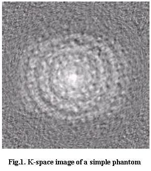
As an illustration of these concepts, Figure 1 shows the K-space landscape of a planar slice of a phantom (i.e., a known and relatively simple test object used instead of a real subject). What is shown in this case, coded by various gray levels, is the magnitude of the complex-valued signal. The individual in-phase (real) and out-of-phase (imaginary) components of the signal would look even more complicated since they assume both positive and negative values. The simplicity of a phantom leads to a relatively simple K-space landscape. The K-space image of something like a human thorax is much more complicated (in fact, nobody but computers ever looks at it). Nevertheless, the basic characteristics listed above are present in both of them. Notice, in particular, how the background noise, here manifesting itself as the disturbing 'grain', makes futile any charting of the K-space terrain beyond a certain distance from the center of the picture. The noise also destroys the symmetry of the K-space landscape (point 3) because it is not bound by equations (1).
There are people who, so to say, feel the pulse of reality even when looking at the K-space images. In the rest of this Section, I want to try and give you some idea about how they do it. You do not need to know the stuff to understand the rest of the Note, though, so if you do not wish to know, feel free to skip it.
Consider first the magnitude of the K-space image at origin. Setting k = 0 in equation (12), we see that Q(0) is equal to the integral of q(r) over the whole volume of interest V. In other words, should I wish to know whether the subject in the scanner is overweight, I would just need to look at the value of Q(0). This insight also tells us that the K-space image magnitude always achieves its absolute maximum right at the origin.
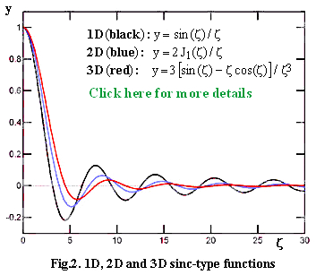
Let us now take a sphere of radius R, full of water, place it at the center of our scanner and see what kind of K-space image we obtain. We know in advance that the image will have a spherical symmetry and, using Eq.(1), we can compute its radial behavior. In this particular case, the imaginary component of the [ideal] signal turns out to be null, while the real component shows a massive central hill surrounded by relatively modest oscillating circular rims. When we plot the normalized shape function against the normalized distance ζ=2πRk, we end up with the same curve for spheres of any size. The graph on the right (Figure 2) shows the shape function for 3D images of spheres, 2D images of discs and 1D images of rods.
The distance normalization to ζ=2πRk means that the smaller is the sphere and the further into the periphery spreads its K-space image (tiny R, large k). Vice versa, a large sphere has its K-space image all peaked close to the origin (large R, tiny k). This falls in line with the general pattern according to which fine-grained details of an R-space image (its effective resolution) are encoded in the peripheral K-space regions, while slow-rolling R-space features are encoded within the central K-space areas. MRI data evaluation software exploits this fact to play sensitivity or resolution enhancement tricks with the images by weighing in different ways the central regions against the peripheral and/or intermediate ones.
One might suspect that the importance of the center of the K-space image arises from the fact that we have placed the sphere at the center of the scanner. It is easy to show, however, that this not so. Let us take an object (no matter what), place it into the scanner and acquire its K-space image, then translate it along a vector d, acquire the new image and see how the two images W(k) and W'(k) differ. From Eq.(1) one obtains
(14)
showing that |W'(k)| = |W(k)| since W(k) and W'(k) differ just by a d-dependent factor which happens to be a complex unity. In other words, translating the imaged object does not modify the magnitudes of the K-space image! What changes is only the balance between the in-phase (real) and out-of-phase (imaginary) K-space components at different points. Likewise, one can easily show that rotating the whole R-space leads to a closely related rotation of the K-space image about its origin and thus, again, does not affect the importance of the central region.
Hopefully, this has given you some feeling for the inner workings of the K-space. Though we have talked just about spheres dislocated in various ways in the R-space, you should consider the fact that any body, however complex, can be well approximated by a sufficiently large number of sufficiently small spheres and that the signals coming from all those spheres are additive.
4. Gradient and pulse echoes
The above observations can be used to elucidate the phenomenon known as gradient echo. Suppose that, upon start, we apply a constant gradient G. In the K-space that makes us fly away from the center at a constant speed in some fixed direction as illustrated in Figure 3a. After some time Δt, we leave the mountains and reach the dull plain with no signal but noise (keep in mind that the signal corresponds to the height of the terrain over which we are flying). At that point, if we invert the sign of the gradient, our velocity will invert sign as well and we shall start backtracking our trail until we reach the mountains again, with a-plenty of signal (thereafter, doing nothing, we are bound to leave the mountains again, this time in the opposite direction). To those who know nothing about K-space, the 'resuscitated' signal may look magic enough to consider it a ghostly echo. We, the seasoned K-space navigators, however, regard such superstitious souls with a pitiful half-amused smile ...
Before your smile becomes an arrogant grin, however, let me tell you something more. It is well known since the dawn of NMR that, in the presence of a field gradient, an echo forms even without changing the sign of the gradient, provided one applies at the time Δt an inversion RF pulse with a nutation angle of 180 degrees. Such an echo is usually called pulse echo or, for historic reasons, Hahn echo). It has one more peculiar characteristic for which there is no analogue in the gradient echo: it is positive when the RF phase of the inversion pulse is shifted by 90 degrees with respect to that of the excitation pulse, but it becomes negative when the phase difference between the two pulses is either 0 or 180 degrees.
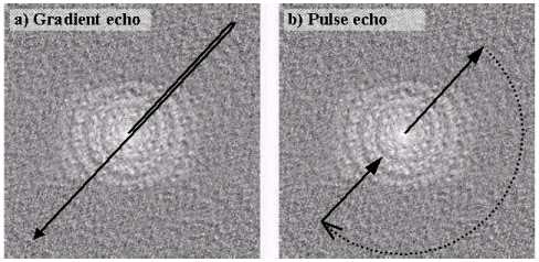
Fig.3. K-space representation of a gradient echo and a pulse (Hahn) echo.
The semicircle is a phenomenological representation of the effect of a 180o RF pulse
(also called inversion pulse or refocusing pulse).
Now, how can we explain that! The fact is that, using just the K-space concepts, we can't. It takes a bit of physics and math to understand why, because of the simultaneous flipping of the magnetization of all the present nuclides, the apparent effect of the inversion pulse is to make our rocket warp through the K-space from wherever it is to a point located symmetrically with respect to the K-space origin. In Figure 3b, the worp is symbolically represented by the dotted semicircle which, however, must not be confused with any real path since the warp is nearly instantaneous and occurs in a spin space which we do not know how to visualize.
Naturally, if the gradient is kept the same all the time, the rocket will keep moving after the warp in the same direction it followed before the warp. Considering the new location, this will carry it back towards the origin where the signal is strong (hence the echo). The final twist is that if the inversion pulse and the excitation pulse have the same or opposite phase, we emerge from the warp below the K-space surface (using the analogy, below the Galactic plane rather than above it) and our consecutive landscape measurements change sign. It is evident that, in general, the 180-degrees pulses enhance our ability to move through the k-space which is why they are sometimes called navigation pulses.
There is one very substantial difference between a gradient echo and a pulse echo which we need to mention here. Since its discovery, the Hahn echo is known to remove the phase-defocussing effects of magnetic field components which are constant during the interval starting with the excitation pulse, including the inversion pulse and terminating with the echo (this is why the inversion pulses are also called refocusing pulses). In particular, one can use pulse echoes to partially remove the detrimental effects of magnetic field inhomogeneity (variations of magnetic field across the sample volume).
Because of the nature of the echoes, such inhomogeneity refocusing occurs only with pulse echoes and not with gradient echoes. We shall return to this point once more in Section 6.
5. K-space charting strategies
There are many ways of approaching the task of charting the K-space - too many to discuss all of them here. However, once we have discussed the principal ones, the reader should have a good idea of the various possibilities and avoid getting baffled by terms like, say, twisting radial lines.
Multi-shot versus single-shot techniques
In order to understand some of the charting dilemmas, we must anticipate the central point of the next Section. The K-space image is transient - it gets re-created after every application of an excitation sequence and then starts decaying back to zero, while the cartographer is desperately trying to complete his measurements.
Fortunately, it is not necessary to chart the whole of the K-space in a single flight. One can repeat the whole MRI excitation-detection sequence many times in what are called single scans or shots, giving the cartographer the opportunity to chart each time a different K-space area. On the other hand, it is evident that single-shot techniques are inevitably much faster which, especially with living subjects, is extremely important.
Kinds of data to collect
Apart from the limited acquisition time, the K-space cartographer is constrained in his work also by the needs of those who will later on use his data to recover the R-space images by means of suitable reconstruction algorithms. It is fairly obvious, for example, that mapping just a few points here and there would not do. However, even when lots of points are collected, covering all K-space regions with a reasonable mean density, the coverage pattern is still important. This is because, at present, there exist fast reconstruction algorithms compatible with just a few coverage patterns and one should stick to those.
The following three categories are at present the most popular ones (for clarity, just 2D versions are shown):
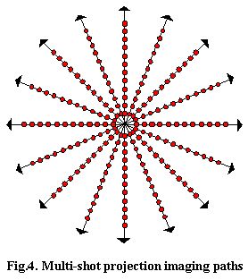
Projection imaging (zeugmatography):
Historically, the radial pattern shown in Figure 4 was the first one to be implemented in clinical practice. In its primitive form, it requires multiple charting flights, each with a different gradient direction while the gradient magnitude is kept constant. During each scan, the sampling rate is usually kept constant (in Figure 4, the sampled data points are indicated by red dots). Using equations (11-13), it can be easily shown that the Fourier transform of each radial array of the collected data corresponds to the projection of the imaged quantity q(r) onto the R-space direction defined by the applied gradient. This is why the approach is often called projection imaging. The complete projection reconstruction algorithms suitable for 2D versions of this technique were initially borrowed from X-ray tomography and other fields and the combination became known as MRI zeugmatography, a term promoted by P.C.Lauterbur.
Due to the radially decreasing coverage density, zeugmatography is characterized by good sensitivity but relatively modest resolution power which borders with uncertainty in distinguishing between certain shapes (the projection reconstruction algorithm can be shown to give unique R-space solutions but just barely so). Because of this, and because of its excessive time requirements, the approach is nowadays rarely used in its original form, but a number of refinements, including single-shot and intermediate techniques, are quite widespread. Some of the obvious modifications include non-uniform sampling (taking more points in the peripheral regions) and/or using gradient echoes to cover two or more radial rays in a single scan.
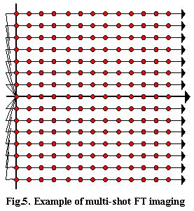
Fourier transform imaging:
The rectangular Cartesian grid illustrated on the right was historically the second charting pattern to be used, promoted by R.Ernst, P.Mansfield and others. The reconstruction algorithm best suited for this case is the Fast Fourier Transform (FFT), closely corresponding to the discrete version of equation (3). Figure 5 shows the grid for just half of the K-space which, due to the K-space symmetry discussed above, is sufficient to define the whole K-space image. The Figure illustrates also a set of possible charting paths but, since there exists a large number of alternatives, the reader should consider these just as an demonstration of feasibility rather than as any binding prescription.
Compared with projection reconstruction, FT imaging assigns more weight to the K-space periphery leading to a much better resolution of fine details, achieved at the price of somewhat lower signal/noise ratio (S/N ratio). Given the uniform coverage density of the Cartesian grid, one can also easily show that the corresponding reconstruction algorithm gives a unique R-space solution with no potential uncertainties. One expects these advantages to apply to any uniform coverage of the K-space. In two dimensions one can in fact conveniently resort to a hexagonal, honeycomb grid for which there exist reconstruction algorithms just as fast as FFT.
In its original version, Cartesian grid sampling appears to be better suited for multi-shot approaches. Nevertheless, many single-shot modifications exist and are in current use. An example of such a single-shot Cartesian grid strategy is the rectangular spiral path shown in Figure 6. One could also use an octagonal spiral covering the same Cartesian grid and hexagonal spiral paths covering honeycomb-like grids. All paths of this kind represents a hybrid between FT imaging and the spiral path strategies to be discussed in the next paragraph.
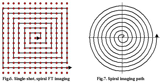
Spiral imaging:
The spiral sampling pattern shown in Figure 7 relies on relatively novel spiral reconstruction algorithms. For simplicity, we have not shown the individual sampling points which are supposed to be distributed at equidistant intervals along the path. In its original version, the radius of the spiral increases linearly with time, the cartographer moves along the path at a constant speed (meaning constant gradient amplitude) and the signal is sampled at a constant rate.
The result is a two-dimensional, single-shot approach with good coverage of the K-space peripheral regions and therefore a good resolution. In its basic version described above, it has also the advantage of considerable technical simplicity. What varies during the scan is just the gradient direction and even that does so in a very smooth way. This reduces to minimum the requirements on the dynamic characteristics of the gradient generators.
As one might expect, a vast multitude of alternatives to the simple spiral had been proposed. Spiraling paths in fact lend themselves particularly well to fancy modifications. One can play with polygonal spirals, vary in fancy ways the pitch of the spiral and/or the data sampling rate, find interesting ways of exploiting the K-space symmetry, etc.
Given the overall good performance of the spiral charting strategies, they constitute at present the fastest growing category. Taking into account the growing accent on single-shot, fast MR imaging (MRI angiography and cardiology), it is likely that spiral-like strategies will eventually completely replace the historic projection- and FT- techniques. In this context, notice that, if need be, a single-shot method can be always used in a multi-shot manner, while the reverse is not true.
There is a lot of on-going work dedicated to finding new and ever faster reconstruction algorithms in 2, 3 and even more dimensions. One even starts hearing about algorithms applicable to arbitrary K-space sampling patterns. That may be an exaggeration since arbitrary is definitely too arbitrary, but it gives one an idea about what are the MRI mathematicians doing these days. In any case, we can expect that, at least from the point of view of sampling strategies, the life of K-space cartographers is going to become ever easier.
Advanced strategies
In the rest of this Section, reserved for the really curious readers who like to know a few little extras, I will try and explain why the idea of nearly arbitrary sampling patterns is, after all, not so haphazard. Consider the following discrete equivalent of equation (3), rewritten for the quantities q(r) and Q(k) in equation (12):
(15)
The integral form of the equation is what theory requires in order to assure a perfect reconstruction. With a finite number of available K-space data, however, integrals can only be approximated. The discrete form on the right, based on a plain summation over the available data points (m=1,2,3,...,N), can be viewed as one such approximation (albeit a rather primitive one). This gives rise to the ubiquitous question of how well can one estimate the value of q(r) using only a limited number of K-space readings.
Though it is not easy to give an universal answer to this mathematical problem, empirical practice shows that, once the K-space symmetry is taken into account, a relatively sparse coverage pattern is enough to produce surprisingly good results. Not only is this true but one obtains reasonable R-space maps even when only limited portions of the K-space are densely covered. There is a deep analogy between the K-space images and holographs. Like in the case of a holograph, a splinter of the K-space image still contains quite a lot of the information required to recover the original R-space map.
The summation formula underlines also the fact that the reconstruction is actually a very simple process. Given a fixed position r in the R-space, every K-space reading of the form {k,Q(k)} contributes to q(r) by a product of Q(k) with the simple complex-unity factor exp(2πik.r). Imagine, therefore, that we choose a grid of fixed R-space points (pixels or voxels) and assign a simple processor to each of them. Now every time we take a k-space reading, we communicate the datum to all the processors who, in parallel, execute the simple calculation required to update the R-space map. With such a multi-processor image reconstruction device, the R-space image is being built in real time and keeps improving even while we are still flying paths in the K-space.
Moreover, it now does not particularly matter whether our K-space data are arranged according to a rigid, pre-defined pattern or not. As long as we keep track of our position in the K-space, any reading is a welcome piece of information and helps to improve the reconstructed R-space map. If efficiency were not a problem, one could even acquire R-space maps from data collected by a completely drunk cartographer flying through the K-space along totally random paths.
Thanks to recent technological advances, in particular the availability of low-cost, high-capacity field-programmable gate arrays (FPGA), real-time reconstruction devices employing large arrays of simple processors running in parallel are becoming an affordable alternative to large CPU's. This technological revolution is still in its early stages, but there is no doubt that it is going to have a large impact on MRI and all but eliminate the need to stick to the old-fashioned single-processor 'fast' reconstruction algorithms.
6. The tyranny of time
We shall now dedicate some time to the transient nature of the K-space landscape, described by the so far neglected decay term in equation (10), namely
(16)
where R2* is the apparent transverse decay rate, inverse of the more-often used apparent relaxation time T2*.
The decay rate in equation (16) contains a number of contributing terms such as the transversal relaxation time, flow effects, self-diffusion effects, spin-coupling effects and - last but certainly not least - the extra de-phasing rate of the signal due to magnetic field inhomogeneity over the whole sample volume. Since the latter term usually dominates, the value of R2* does not vary much from point to point and equation (10) is usually well approximated by
(17)
Even when such approximation is reasonable, the transient character of the NMR signal still represents a vexing problem for our K-space cartographer who now has to map an area in which whole ranges of mountains periodically flicker into existence and then decay into a dull plain. Evidently, this leaves him with no time to spare and introduces a number of logistic and computational problems. One needs charting strategies which, apart from the paths to follow, carefully take into account the times needed to cover them.
We shall now discuss a few aspects of this problem. Some of these aspects border on research topics and thus exceed the scope of this Note. Nevertheless, the following generic reflections may be essential for those readers who want to understand not just the principles of the K-space description but also its limitations and practical applicability.
Speedy charting
One possible approach to the difficult task of charting transient landscapes is to do the job so fast that the decay can be neglected. When the whole charting job is done in a time period Δt such that the decay factor (16) remains close to 1 during the whole charting process, it can be neglected and one can proceed exactly as we have done in preceding Sections. This, however, is easier to say than to do. There are two types of objections to such an approach.
The first category of objections is purely technical. Whatever charting strategy is used, the faster we wish to move through the K-space, the more powerful 'motors' we need. In our case, this means more powerful, responsive and reproducible dynamic field gradient generators (including the gradient coils and the respective current sources). This translates into high equipment costs and high average power consumption (operating costs). To stay with our analogy, if you wish to move real fast, a Ferrari may be still too slow; what you need is an executive jet, but then you have to pay for it.
The technological limits become even more stringent when one is after single-shot charting strategies. To obtain a reasonably dense chart of the whole K-space following a single path, the latter must be necessarily very long and curvy and, in order to be reproducible, also very precise. If, in addition, the job must be done in a short time, this implies speeds and maneuverability considerably superior to whatever might be acceptable for multi-scan strategies.
The second category of objections has more to do with physics. For reasons of very fundamental physical nature, NMR is always characterized by a relatively low signal-to-noise ratio (limited sensitivity). It is therefore imperative to collect all the available signal and not throw away any of it. Which, however, is exactly what we are doing when trying to finish the charting before any appreciable decay takes place. Once we have finished, there is still a lot good signal but we ignore it just because it has already decayed a bit and we are too lazy to complicate our lives by accounting for the decay in our evaluation algorithms.
Another aspect which is closely related to the sensitivity problem is the sampling rate. According to a Nyquist theorem, the required receiver bandwidth is equal to the rate at which one samples the signal. Fast sampling implies large receiver bandwidth which, in turn, implies more receiver noise (the variance of the latter is proportional to the bandwidth). Consequently, the combined effect of reducing the charting times and, consequently, increasing the sampling rates brings us eventually to a situation where the quality of the recovered images becomes totally unacceptable.
Slowing the decay
If the decay is such a problem, are there not ways to get rid of it or, at least, slow it down? The answer is there are, though they may be costly and work only up to a certain point. We have said that the decay is usually dominated by the magnetic field inhomogeneity over the whole imaged volume. There are two ways how such an inhomogeneity can be reduced:
(1) Building more homogeneous magnets and, just as important, making sure that the environment in which they are installed does not compromise their homogeneity. However, better homogeneity is a technological challenge and its solutions come at a cost. Thus a magnet with 3 ppm (part-per-million) inhomogeneity over a certain volume may cost several times more than one with 30 ppm over the same volume.
Apart from the costs, there are also intrinsic limits to this approach. The imaged objects are normally very heterogeneous (this is certainly the case with human bodies) and thus, due to magnetic susceptibility differences between their constituent parts, generate induced magnetic field inhomogeneity of the order of a few ppm even in perfectly homogeneous external magnetic fields.
(2) Reducing the imaged volume. The smaller is the imaged area, the smaller is the field inhomogeneity across it and, as an extra bonus, the fewer data points are needed to chart it. These are the two reasons for using local RF coils which pick up only signals arising from a limited area of a larger body. Hence the existence - and the often excellent performance - of local coils for limbs, shoulders, spine, cervix, rectum, prostate, testicles, eyes, etc, etc.
One can take this approach a step further. If we could split the whole imaged volume into smaller compartments, each monitored by its own pick-up coil, we might end-up with a composite image of the whole volume and a quality corresponding to the size of the partial volumes. Due to the nonlinear, exponential behavior of the decay term (16), this leads to very substantial gains in quality and/or reductions of total scanning time and lies behind the idea of using arrays of local coils, each with an independent receiver channel.
Numeric corrections
There is one rather obvious thing one can do while evaluating the acquired data. To the extent to which the decay rate in equation (16) is independent of position and equation (17) is justified, it can be accounted for and corrected a-posteriori. All we need to do is to
(a) a-priori estimate the decay rate and
(b) while charting the K-space, complement each reading with the time at which it has been taken (starting from take-off at t=0).
This technically simple modification (time readings are among the most simple ones to take) leads to data triplets of the form {k,Q'(k),t} in which Q'(k) is the partially decayed value of Q(k). When t and R2* are known, it is then elementary to recover Q(k):
(18)
Compared with what we have called plain speedy charting, inclusion of time in data logs and usage of equation (18) can help to extend the tiny time windows useful for K-space charting by a factor of two to three which, when all numerical estimates are made, may amount to almost tenfold reduction of the total scanning time needed to obtain an image of a given quality.
Beyond that, however, things start getting worse rather than better. The reason is that the correction factor in equation (18) is always greater than one and grows exponentially with the elapsed time t. Consequently, it not only corrects the decay but also amplifies the receiver noise. As we push equation (18) to ever longer times t, therefore, there comes a point where further improvements in artifacts become marginal while the noise starts getting out of hand.
Decay versus apodization
One can ask what would happen to the final R-space images if one simply ignored the presence of the decay factor (16). It so happens that the answer to that question depends a lot upon adopted K-space charting strategy. Before giving the actual answer, however, we need to introduce a widely used data-evaluation concept.
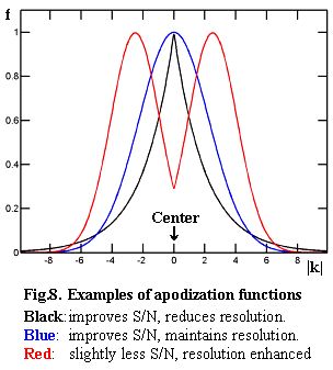
We have already mentioned the fact that the reconstruction software can play with the relative weights of the central, intermediate and peripheral regions of the K-space in order to modulate R-space signal-to-noise ratio and/or resolution. In general, this is done by multiplying the K-space image by a function f(|k|) which depends only upon |k| but not upon its direction. The process is known as K-space weighing or K-space apodization and corresponds closely to an analogous procedure routinely used in NMR spectroscopy as well as a number of other fields, unrelated to NMR. Figure 8 shows three typical apodization functions and gives a clue about their effects.
Returning to the decay factor (16), we notice that, combined with some of the K-space charting strategies, it affects the K-space image in a way similar to an exponential apodization function f (like the black one in Fig.8). This is exactly the case, for example, when applying the multi-scan projection-imaging and, to a good approximation, when using one of the spiral strategies. In such cases, the general effect is an extra suppression of the peripheral K-space signal and thus a reduction in spatial resolution. Unlike a-posteriori exponential apodization, the suppression of peripheric signals is not accompanied by any noise reduction and therefore does not improve the image signal-to-noise ratio. The only consolation is that, in these relatively lucky cases, the effect at least does not introduce any image artifacts.
Unfortunaley, there are many K-space charting strategies in which the decay factor affects the data in an a-symmetric way. In the case of the multi-shot FT imaging shown in Figure 5, for example, the apodization effect due to the decay is much more pronounced along the X-axis than along the Y-axis. Such a-symmetries are bound to generate fastidious artifacts in the R-space images (single/multiple ghost images, smeared images, ...). In particular, one must avoid strategies in which the effective decay-induced apodization function might contain any sharp discontinuities.
In most cases (certainly all the 2D ones) it is possible to correct the decay artifacts by repeating the whole data acquisition several times, rotating each time the whole K-space image by an angle and properly summing together all the partial data. For example, the multi-shot Fourier-transform data acquisition can be repeated rotating the whole charting pattern by 90 degrees and then summing the two distinct signal values obtained for each data point. This removes the X/Y a-symmetry leaving just a modest eight-fold azimuth angle dependence. Symmetrization procedures of this type are very effective and lead to efficient artifact suppression once at least a four-fold symmetry can be guaranteed. Exploiting the inversion symmetry of the whole K-space, the four-fold symmetry can be reached with just two scans (4 scans for an eight-fold symmetry etc).
Exploiting pulse echoes
The ideas of the preceding Section can be taken one step further by an ingenious exploitation of gradient echoes. For example, one can mitigate the differences due to signal decay along a path by backtracking it and summing the readings taken at the same points but at different moments. In this way, it is possible to modulate in many various ways the effective apodization function due to the decay factor (16). Since the decay factor is dominated by static field inhomogeneity, however, and since the latter is not refocused by gradient echoes, the overall total loss of signal intensity is always the same. One can at best distribute it in different ways among different areas of K-space but not remove it.
Moreover, the static field inhomogeneity is a-specific in the sense that it is mostly a characteristic of the instrument and not of the imaged subject. The signal decay therefore can not be exploited to obtain any knew contrasts between tissues. On the opposite, whatever differences there might be, it tends to mask them and thus attenuate contrasts in the final R-space images.
On the other hand, we know from Section 4 that pulse echoes do remove the static field inhomogeneity. This means that, for example, the pulse echo shown in Figure 3b should be substantially stronger than the gradient echo of Figure 3a. It turns out that not only is this indeed so, but the intensity of the refocused echo decays with a rate which, after the removal of the dominant a-specific term, depends upon intrinsic characteristics of the imaged tissues, such as the transversal relaxation rates and water diffusion coefficients.
This explains why pulse echoes are of extreme importance in MRI. They help us combat the field inhomogeneity and, at the same time, give us the possibility of introducing new, tissue-specific factors into the acquired images.
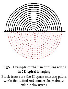
Since this treatise has become much longer than what I had initially in mind, however, I am not going to pursue this topic much further. The reader can by now imagine that there are hundreds of clever schemes of incorporating the pulse echoes into the K-space charting process. Perhaps the best thing is to conclude with a single, slightly fancy example illustrating one of the almost infinitely many ways how the pulse echoes can be used. Though I do not think anybody is using this method yet, it should be pretty good.
Figure 9 shows what is essentially a single-shot, spiral path, except for the fact that the lower half-plane lobes of the spiral are replaced by spin-echo warps. To assure proper refocusing while maintaining constant charting speed, a little timing trick needs to be added. If we index the lobes 1,2,3, ... (starting from the innermost ones), we insert a small, constant time delay before starting to traverse the odd lobes, while no such delay is applied to even lobes. The purpose is to make identical, for every single k, the time needed to complete lobe 2k and 2k-1. In this way static field inhomogeneites get refocused within every pair of lobes and the overall signal decay is dominated by the much slower transversal relaxation rate (plus any diffusion effects).
7. Concluding remarks
The reader who has followed this exposition should know quite a lot about how MRI images are formed. This, however, is only one aspect of MRI. We have not talked about the actions which need to be taken before the acquisition of MRI data can start. In particular, this includes
- preparation of nuclear magnetization (preparatory pulse sequence),
- nuclear magnetization excitation by a suitable RF pulse (non-selective, selective, profiled), and
- sensitive manifold pre-selection (plane, multi-plane, line).
The three tasks are closely related and often intricately interconnected. They are achieved by means of suitable RF pulse and field-gradient sequences. In this respect, too, MRI is characterized by an amazing multitude of choices which affect, often quite strongly, the nature of the imaged quantity q(r) and the way it depends upon all the parameter at play (spin density, longitudinal and transverse relaxation times, diffusion and flow). The theories behind these aspects of MRI experimental techniques were not discussed because they are of more traditional NMR nature and rarely invoke the K-space concepts. For the same reason, we have just listed some of the phenomenological features of pulse echo, avoiding any in-depth explanations.
I have refrained from a systematic exploration of all possible combinations of K-space charting strategies, image reconstruction schemes and of the many ways of using gradient and spin echoes. Apart from the fact that the total number of potentially interesting approaches is staggering, I doubt whether, at present, a systematic review is possible (or even makes sense), since many technical aspects of the problem (such as the massive parallel processing techniques) are still in rapid evolution.
I have also omitted the discussion of motional and other artifacts and flow effects. Likewise, I have skipped the k-space description of those MRI techniques which employ heavy RF pulse trains during data acquisition (such as steady-state free precession and pseudo-stochastic methods). The discussion of such topics within the k-space formalism, though still convenient, assumes aspects which go beyond an introductory exposition. Those interested in such topics should look them up in the references listed below and consult the original literature.
Naturally, many special aspects of K-space were just barely mentioned, avoiding dozens of mathematical theorems. I have tried to stress the inherent simplicity of the K-space description while, at the same time, letting transpire the versatility of the formalism and the staggering number of possible solutions which make MRI still so attractive to physicists and mathematicians.
Occasionally, the exposition has been pushed up to the frontiers where active research is going on.
Hopefully, this might help a few new adepts to plot the direction of their future efforts.
|