|
Introduction and definitions
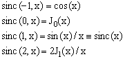
The sinc(x) function,
(1) 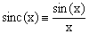 , ,
is often encountered in physics and engineering. It comes up in all problems involving, directly or indirectly, the Fourier transform of a quantity distributed uniformly over a finite interval. In particular, if a property P has a uniform value p over the interval [-R,R] and zero everywhere else, its Fourier transform is
(2) 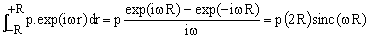 , ,
Likewise, it arises also when asking about the power spectrum of an excitation which is gated On/Off in time (pulsed stimulus such as, for example, the radiofrequency pulses used in NMR).
Considering that a real numbers interval may be interpreted as a one-dimensional sphere, formula (2) can be generalized to n-dimensional problems. Let
(3) 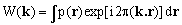 , ,
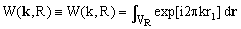
be the n-dimensional k-space representation of the distribution p(r) of the property P. Here the integral is taken over an n-dimensional Euclidean space, k = {k1,k2,...,kn} and r = {r1,r2,...,rn} are n-dimensional vectors. We now assume that p(r) has the distribution
(4) p(r) = 1 when |r| ≤ 1 and p(r) = 0 otherwise.
To distinguish this special case, we will use the notation W(k,R) instead of just W(k). Notice that the constant value of p(r) inside the sphere of radius R does not limit the generality of the discussion since, were the value some p, our W(k) would be proportional to it and, since we will eventually normalize, it would cancel out.
The evaluation of W(k,R) is greatly simplified by the symmetry of the distribution of p(r). For any direction of k, it is always possible to rotate the Cartesian coordinate system so as to make k co-linear with the first axis, i.e., k = {k,0,...,0}. Since the value of the integral does not depend upon the choice of the coordinate system and since any rotation leaves invariant the spherical distribution of p(r), we see that W(k,R) depends only on the magnitude k of k and not on its direction. It therefore remains to determine just its radial profile W(k,R).
Choosing k = {k,0,...,0}, equations (3) and (4) give
(5)  , ,
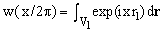
where the integral is taken over the volume VR of the n-dimensional sphere of radius R centered at origin. We can scale r to normalize the integration volume, setting r = Rr', r1 = R r1' and dr = Rn dr'. Then
(6)  , ,
where we have set x = 2πkR, and the integration extends over the volume V1 of a sphere of unit radius.
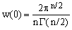
It is evident that W(0,R) is the volume of an n-dimensional sphere of radius R and that, due to the scaling properties, the ratio W(k,R)/W(0,R) depends only on x. We can therefore define a function of x such that, for any value of R,
(7)  , ,
where w(k) = W(k,1).
Equation (7) is our generalized definition of the sinc(x) function pertinent to n-dimensional Euclidean space. It can be described as the normalized radial profile of the Fourier transform of uniform n-dimensional sphere with unit volume. It is easy to verify that for n = 1, this definition coincides with equations (1) and (2).
Using sinc(n,x), the radial profile W(k,R) of the Fourier transform of a homogeneous n-dimensional sphere of diameter R (eq.5) can be written as
(8) 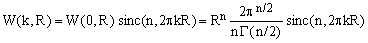 , ,
Here we have used the explicit formula for the volume W(0,R) of an n-dimensional sphere derived in [ref.2, eq.22].
Closed form expressions for sinc(n,x)
To evaluate sinc(n,x), we will use the second form of Eq.(7) and the results obtained in [2].
The volume of an n-dimensional sphere of unit radius is known to be [ref.2, Eq.22]
(9)  , ,
where Γ is the gamma-function. We therefore need to concentrate just on the integral
(10)  , ,
over a sphere V1 of unit radius. Using the series expansion of the exponential, one obtains
(11) 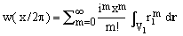 , ,
Due to the symmetry, the integrals in the terms with odd powers of x evaluate to zero.
Hence, setting m = 2s, we have
(12)  , ,
The integrals appearing in Eq.(12) are known for any n-dimensional ellipsoid [ref.2, Eq.20].
In our special case of a unit radius sphere,
(13) 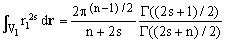 . .
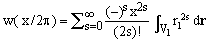
Combining Eqs. (7), (9), (12) and (13), one obtains the following series expansion:
(14) 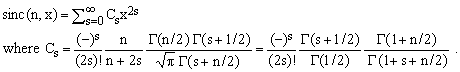 . .
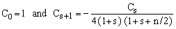
This looks a bit formidable but it can be simplified using the identities [3,4]
(15) 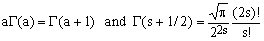
and isolating terms which are independent of s. One thus obtains
(16) 
Comparing the series with the expansion formula for Bessel functions of the first kind [3-7],
one verifies that
(17)  , ,
so that, finally
(18) 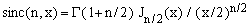 . .
The family of sinc(n,x) functions of Eq.(7) is therefore closely related to half-integer Bessel functions of the first kind.
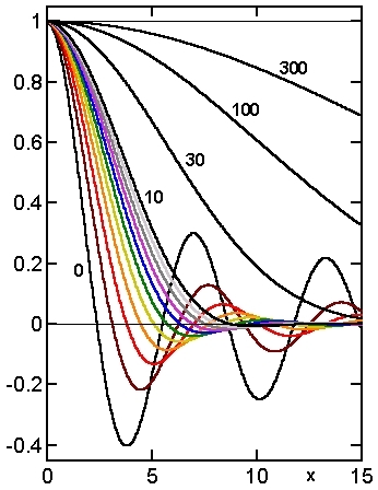
Figure 1. Graphs of selected functions sinc(n,x)
Since the functions are even, they are shown only for x ≥ 0.
Codes: n = 0 (black), 1 (brown), 2 (red), 3 (orange), 4 (yellow),
5 (green), 6 (blue), 7 (violet), 8 (gray), 9 (silver), 10 (black).
All black curves are labelled with their values of n.
Generated by a simple Matlab program.
Numeric calculations and graphs of sinc(n,x)
Brute force numeric evaluations of the power series expansion (14) can be carried out exploiting the recurrence relation
(19)  . .
This works well for modest values of the argument x (up to about 30) and is especially recommended when x < 2. For larger values of x rounding errors ruin the results and it is preferable to use Eq.(18) and apply one of the many known methods for the calculation of Bessel functions.
The Figure on the right illustrates some of the following features of the sinc(n,x) functions: Due to construction, they are all even functions with value 1 at x = 0. For n > -1, they approach 0 when x goes to infinity (in physically meaningful contexts they are decaying transient functions). They all exhibit damped oscillations and have an infinite, countable set of roots. With increasing n, corresponding roots shift to ever higher values and the amplitude of the oscillations decreases (in particular that of the first negative lobe). Around n = 10, the oscillations become too small to be physically meaningful (even though they are still present).
Extensions, recurrence relations and special cases
The physical problem with which we have started makes sense only for integer n > 1. However, Eq.(18) makes it possible to extend the definition to any real-valued n, excluding only negative even integers for which the Γ(1+n/2) is undefined.
Applying the well known recurrence relation for Bessel functions,
(20) 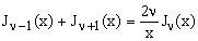 , ,
one derives the following recurrence for the sinc(n,x) functions:
(21) 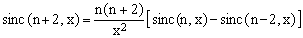 . .
This splits the sinc(n,x) functions in two separate recursive progressions - one for even n and one for odd n - each of which needs two starting terms. Using well known trigonometric expressions for J-1/2 and J1/2, one finds
(22) 
which can be used to start the recursions of Eq.(21), obtaining
(23) 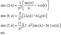
All the sinc(n,x) functions with even n can be therefore expressed in terms of J0(x) and J1(x), while all those with odd n can be expressed in terms of sin(x) and cos(x).
The recurrence formula (21) gives us also an insight about what happens for negative values of n. While sinc(-2,x) is undefined, the function sinc(-3,x) = cos(x)+x sin(x) exhibits divergent oscillations rather than damped ones. The break-even occurs at n = -1; sinc(-1,x) = cos(x) is in fact neither damped, nor diverges.
Roots of sinc(n,x)
For the physically most significant cases of n = 1, 2, and 3 the roots of sinc(n,x), henceforth denoted as ξn(m), m = 1, 2, 3, ..., have a particular significance due to the fact that, according to Eq.(8),
(24) 
for some m. In many applications - such as magnetic resonance imaging - the W(k) values are experimentally accessible so that determining the k for which they become null permits an estimate of the radius of the imaged sphere. From this purpose, the most important root is the very first one (m = 1).
A simple inspection shows that:
| ξ-1(1) |
= 1.570 796 326 794 ... = π/2 |
... is the first root of cos(x) |
| ξ0(1) |
= 2.404 825 557 695 ... |
... is the first root of J0(x) |
| ξ1(1) |
= 3.141 592 653 589 ... = π |
... coincides with the first non-zero root of sin(x) |
| ξ2(1) |
= 3.831 705 970 207 ... |
... coincides with the first non-zero root of J1(x) |
| ξ3(1) |
= 4.493 409 457 909 ... |
... is the second non-zero solution of tan(x) = x |
| ξ4(1) |
= 5.135 622 301 840 ... |
... is the first non-zero solution of 2J1(x) = x.J0(x) |
All these constants occur quite frequently in various contexts of mathematical physics and engineering.
Combining their values with Eq.(24) we see that for the one, two and three dimensional cases 2R = 1/k, 1.22/k, and 1.43/k, respectively. The relationship between the first zero of W(k,R) and the diameter 2R is well known for the 1D case, but the 2D and 3D cases are rarely mentioned and the fact that there is a significant numeric difference between 2R and 1/k is little known.
|