|
I. Introduction
Let [a,b] be a real-numbers interval of length Δ = b - a, y(x) a linear function of real variable x and r a real or complex constant. Then, using the elementary indefinite integrals
(1) 
one can easily show that
(2) 
where
(3) 
Suppose now that {xk}, k = 0,1,2,...,n, is a sequence of increasing real numbers, write Δk = xk - xk-1 for any 0 < k ≤ n, and let y(x) be a polygonal function (or P-function) composed of linear segments connecting the adjacent points (xk, yk), yk = y(xk). Then Eq.(2) gives
(4)  . .
A special case arises when the points {xk} are distributed uniformly and Δk = D for all k. In the following we will refer to the polygonal functions defined over a uniformly distributed array of points {xk} as UP-functions. According to Eq.(4), the exact exponential integral transform of a UP-function y(x) is
(5)  , ,
where
(6)  . .
II. Comparison with other numeric integration formulae
When r = 0 we have h = 1/2 and equation (3) reduces to the well-known trapezoidal integration rule [1].
For non-zero r-values, a direct application of the trapezoidal rule [1] to the complete integrand on the LHS of Eq.(5) gives the approximate expression
(7)  . .
where O{} is the residual-error approximation.
Equations (5) and (7) can be both used for numeric integration of tabulated functions or experimental data arrays. Since equation (5) is exact for polygonal functions while Eq.(7) is not, one expects Eq.(5) to give better results than Eq.(7) in those cases where polygonal approximation of y(x) is better than that of e-rxy(x).
Equation (5) differs from the trapezoidal formula by the fact that the naive numeric transform represented by the summation term is multiplied by the factor χ(rΔ) which depends upon r and that, in a similar way, the correction terms for the first and last points are r-dependent.
Being defined on a uniform grid, Eq.(5) resembles the Cotes-Newton integration formulae [1,2]. On the other hand, since it involves an exponential weighting function, it resembles also the approximations belonging to the Gauss-Legendre family [2]. In this sense we might say that, as an approximation, it is a hybrid type combining some aspects of each of the two families.
III. Special cases
Equation (5) is valid for any real or complex UP-function and any complex r.
When r is real and positive, it represents an explicit expression for the Laplace transform of the polygonal function y(x).
When r = -iω, it becomes an explicit expression for the Fourier transform of the polygonal function y(x).
In this case η(rΔ) = η(-iωΔ) is complex and χ(rΔ) = [χ(iωΔ)+χ(-iωΔ)] is real (both quantities are ω-dependent).
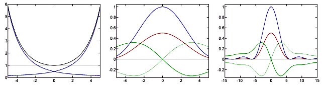
Figure 1. Graphs of the functions η(x), χ(x) against x and η(iω), χ(iω) against ω
generated using a simple Matlab program.
Left: blue: η(x) (decreasing) and η(-x) (increasing), black: χ(x).
Right: same as middle but for a broader range of ω-values.
Center: blue: χ(iω), red: Real(η(iω)) = Real(η(-iω)), green: Imag(η(iω)) (bold) and Imag(η(-iω)) (thin).
IV. A special-case Fourier transform theorem
When r = -iω and ωΔ = 2πk, k being a non-zero integer, then χ(rΔ) = 0, η(rΔ) = i/(2πk). It follows that, for any UP-function defined on such a grid,
(8)  . .
In other words, when D is an integer multiple of the period of the function exp(-iωx), the value of the Fourier integral does not depend upon the path which the UP-function y(x) follows between the extreme points and it is zero when the y(x) values at the extreme points are the same.
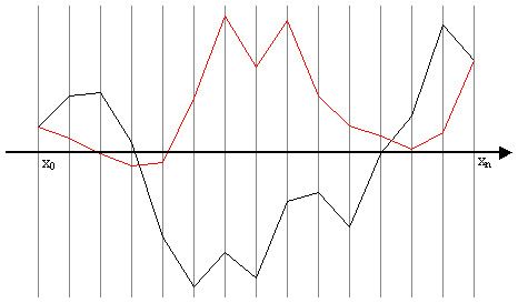
Figure 2. Illustration of Identity (8).
When ωΔ = 2πk, the Fourier integrals of the two UP-functions (black and red) are exactly the same.
This statement is a sweeping generalization of the fact that the integral of any harmonic function vanishes over an interval whose length is an integer multiple of its period. It has a number of practical corollaries in applications using Fourier transforms of functions which can be approximated by UP-functions.
A discussion of such corollaries will appear elsewhere.
|