1. Introduction

Analog electronic devices are made to handle electric signals. Unfortunately, all electric signals contain a certain amount of noise and all devices which handle such signals add some amount of noise of their own [1-5].

In this Note we shall consider only unbiased noise, i.e., one whose mean value is zero. This need not be necessarily true but, whenever it happens, the mean value is best interpreted as a systematic bias or as an input offset and handled by non-statistical means.

An unbiased random noise e(t) is primarily characterized by means of its variance

(1),
where <x> denotes the mean value (average) of x, e² is the noise variance and e is its root-mean-square (rms) amplitude which, in the case of normally distributed noise, coincides with its standard deviation.

Random functions of time have many other characteristics, but we are not going to need them here. For what regards the physical type (dimensionality) of the noise, one usually intends noise voltage but there are many devices (such as current amplifiers) for which it is more natural to consider noise current. Here we will start with voltage noise and only later discuss the closely related current noise.

Every electronic device has a reasonably well defined frequency band and the variance of any noise e(t) associated with the device depends upon the width Δf of the band [5]. Imagine that the band is divided into narrow frequency slices. It is then as though the total noise were the sum of components arising from the distinct slices. Having different frequencies, all such components are almost inevitably statistically independent and, consequently, their variances add up linearly. It follows that when the noise in all frequency slices has the same amplitude, the variance of the noise from the whole band is proportional to Δf. In order to get rid of this dependence, one defines a quantity called spectral noise density n as

(2).

In practice even the noise density often depends upon frequency but, when it does, the dependence - being purged of the obvious linear factor - represents a physically significant phenomenon.

Data sheets of electronic devices always report noise densities rather than noise rms amplitudes and express them typically in nV/√Hz for voltage noise and pA/√Hz for current noise.

2. Signal and noise propagation through an electronic device

Most electronic devices, both active and passive, transform an input signal into an output signal. Among these, there is a large category of linear devices in which, under a broad range of conditions, the output is proportional to the input. In such cases, the proportionality constant is called either gain or attenuation, depending upon whether it is greater or smaller than 1, respectively. Since there is no conceptual difference between these two classes, we shall denote the constant as G and call it gain regardless of whether it is smaller than, equal to, or greater than 1.

Many linear electronic devices have a variable gain. In such cases it is very common that the output noise, just as the output signal, is proportional to the selected gain. In passive devices, such as resistive voltage dividers, this has a nearly obvious justification. In others, such as linear amplifiers, it is an approximate empirical fact (see the box on the right for an indirect reason for why this happens). In all cases, it is a good idea to think about the output noise as though it were due to a somewhat hypothetical input noise, multiplied by the gain factor G. In this way one ends up with an input noise specification which is nearly independent of the selected gain. For the sake of uniformity, we apply this kind of normalization to all devices, regardless of whether their gain is fixed or variable.

It is further necessary to consider the dependence of the input noise obtained by means of the above recipe upon the noise which is present in the input signal already before reaching the electronic device. Clearly, we expect the two to be related. Should the signal noise be very large, we expect the device to amplify it in the same way as the signal, but otherwise to leave it practically unaltered. It turn out, however, that this is impossible when the noise in the external input signal is smaller than some device-dependent limit. The situation is usually modeled by assuming that the variance of the device input noise is the sum of the variance of the input signal noise plus a device-dependent constant. The latter can be interpreted as the variance of an equivalent input noise generated within the device and statistically independent of both the signal and its noise.

Summing up what has been said so far, the noise characteristics of an electronic device are generally modeled according to the schematic diagram in Figure 1. The legend of this Figure also lists and defines all the quantities which will be used in the rest of the text.
 

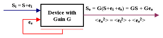
Figure 1. Signal and noise propagation in a linear electronic device with gain G.

The input signal S_i is composed of the 'true' signal S and the random input noise e_i. The device generates a noise of its own, summarized by the equivalent input noise e_e (the red lines are a reminder that e_e actually models noise generated throughout the whole device). The input signal S_iand the equivalent input noise e_e, summed together and multiplied by the gain G, give rise to the output signal S_o, composed of the 'true' signal GS and the output noise Ge_o, where e_o = e_i+e_e. Since the two noise components are uncorrelated, the variance of e_o is the sum of the variances of e_i and e_e. All signals shown here are functions of time; we have just dropped the superfluous (t) indication.

3. Input and output S/N ratios

From the above diagram one easily obtains the relation which links among themselves the output and input signal-to-noise ratios. For simplicity we will still use the same symbols as before to denote the various noises but from now on they will no longer indicate random time function but their rms amplitudes. Accepting this convention, one obtains

(3).

In the last passage we have exploited Eq.(2) and the fact that the input bandwidth of the device for the signal and for the equivalent input noise are supposed to be the same. This makes it possible to express the factor under the square root in terms of spectral noise densities, n_e and n_i, rather than the rms noise amplitudes.

The term in the leftmost ellipses is of course the output signal-to-noise ratio while the one in the rightmost ellipses is the input signal-to-noise ratio. Symbolically, we shall denote these quantities as (SN)_out and (SN)_in.

The input/output ratio f between the two SN ratios,

(4),

depends only upon the ratio between the spectral densities of the equivalent input noise of the device and the noise actually present in the input signal.

Keep in mind that, despite the approximate normalizations we have done, the equivalent input noise density may still depend upon center-band frequency - especially when the latter varies over several orders of magnitude. It is also likely to depend upon the device temperature and, in some cases, it may depend also upon its input impedance and/or output load. Occasionally, plots of such dependencies appear in the data sheets of various commercial devices. Consequently, the factor f also exhibits all such dependencies.

Knowing the equivalent input noise density of the device and the noise density of the signal, Eq.(4) makes it easy to estimate the noise density of the output signal. However, since the factor f of Eq.(4) depends also on the input noise, it is not a unique characteristic of the device and therefore may not be confused with the device noise factor. To arrive at that, we have to introduce another level of normalization - a matter which will be discussed in the next Section.

4. Noise figure of a device

Many devices used for frequency bands ranging from audio-frequencies to microwaves [6] are built to match pre-defined input and output impedances. This makes it easy to interconnect them in various combinations, using standard-impedance connection lines (from twisted pairs and coaxial cables up to waveguides).

When a device has a well-defined, resistive input impedance R, its input is normally connected to another device or sensor of the same output impedance. This imposes a lower limit on the input noise which can not be smaller than the Johnson thermal noise on a resistor of the same value. Considering that the latter is given by the well-known formula

(5),

where T is the absolute temperature in degrees Kelvin [7] and k is the Boltzmann constant [8], it follows that

(6).

The expression on the right-hand side of the above equation depends exclusively upon device characteristics and it is this worst-case f-ratio which defines the noise figure of the device. Since f is a dimensionless ratio of voltages, it is normally expressed in decibels [9] and denoted as F

(7).

This is the formula which relates the equivalent input noise density of a device to its noise figure. It follows that in order to define the noise figure, unlike the more general equivalent input noise density, one must know the input impedance of the device and the temperature at which it operates. Many textbooks overlook the necessity to stress this fact, causing quite a bit of confusion in student's heads.

It is evident from equation (7) that F is always a positive quantity. Its typical values range from < 1 dB (excellent) to a few dB (medium) to >10 dB (rather bad). It is easy to invert the formula and determine the equivalent input noise density from the noise figure:

(8).

For F= 1 dB and a 50 &Ohm; device at room temperature (298 °K), for example, this gives n_e = 0.326 nV/√Hz.

5. Equivalent input current noise density

For devices with a pre-defined input impedance R it is possible to define also the equivalent current noise density j_e.
Since this is related to n_e by the elementary formula

(9),

equations (7) and (8) can be rewritten as

(10),

and

(11),

For the above example of F= 1 dB and a the 50 &Ohm; device at room temperature (298 °K) this gives j_e = 6.52 pA/√Hz.