|
Ad Astra Ltd and Early History of Gravity Engineering
|
This educational article presents a slightly amusing simple instance of variational calculus. It also discusses some of the applied aspects of the presented problem which purports to regard the foundation of would-be gravity engineering, intended as a branch of space engineering. To appreciate it, you must think in terms of building large mansions in deep space - large enough to possess a few percent of the mythical and half-forgotten Earth gravity - and doing so at prices affordable to a sufficiently large number of wealthy communities.
|
|
Preface
Since a long time I have felt the urge to describe the great achievements of my grand-grandfather whose mathematical acumen provided the competitive edge to the Ad Astra Enterprise, Ltd, which, as everybody knows, was founded by my grandfather and is today the largest civil engineering Company in the Solar system. I particularly wish to dispel the rumors according to which the Company's success is due exclusively to my grandfather's murky financial deals. It is true, of course, that my grandfather has shown the Arabs a way to recycle in Space Engineering the petrodollars they have amassed when petrol still existed. It is also true that my father married an Arab Emirates princess and embraced the Prophet. It may be that without these events, Ad Astra would today not be what it is. However, while all this may be true, it is absolutely certain that Ad Astra would have never gotten off the ground without the math of my grand-grand-daddy.
The funny thing about all this is the fact that the said math is by no means complex. Today, it is taught at many colleges and even in my grand-grand-daddy's time it was within the reach of undergraduate sophomores majoring in any of the natural sciences. Sometimes, great discoveries lay right in front of our eyes and yet we fail to see them.
What follows are transcripts of my grand-grandfather's surviving notes (a kind of hand-written mess, really) and of the reminiscences of my grandfather jotted down in the rare moments when he was somber (may Allah have mercy with his soul). From the notes it transpires that my grand-grand-daddy Stan was an impractical man quite unaware of the fact that his equations could one day become a source of revenue. Or, if he was aware of it, he did not care.
I take the liberty of commenting on the notes but, in order not to confuse my comments with the original material, they are set in a different type on a colored background.
|
|
Formulation of the problem
Let us consider the following problem:
We have at our disposal a certain amount of matter with specific density η and volume V. This amounts to the mass M = ηV capable of generating gravitational attraction. Now suppose that we wish to use this matter to construct an object which, at one point of its surface, attracts small material objects with a maximum possible force.
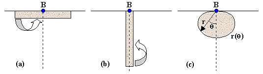
Figure 1. Getting maximum gravity from a fixed amount of matter.
A given amount of matter of constant density is to be arranged so as to maximize the gravity at a barypole B. The matter will have to be located all on one side of a baryplane passing through B which we imagine perpendicular to the image (the solid horizontal line is its footprint). The horizontal disk (a) and vertical column (b) arrangements are not optimal since a transfer of a small amount of mass indicated by the arrows increases the gravity at B. The optimal solution is an axially symmetric body like the one shown in (c) whose optimal contour curve r(θ) needs to be determined.
One feels that all the mass should be located on one side of a plain passing through the point of maximum attraction because otherwise the gravitational forces due to the masses located on different sides would partially cancel each other. We will call the point of maximum attraction the barypole and the plain passing through it the baryplane. Now, if the matter were arranged in a flat disc adherent to the baryplane as shown in Fig.1a, much of it would be located along the rim of the disc, too remote from the barypole to be effective. Equally unsatisfactory would be an arrangement along a long rod perpendicular to the baryplane (Fig.1b).
In both cases, in fact, one just needs to take a piece of the material lying far away from the barypole and move it somewhere closer in order to increase the gravity at the barypole and thus prove that the arrangement is not optimal. For an arrangement to be optimal, it must be impossible to increase the barypole gravity it by any transfer of material from surface location to another.
It therefore appears that the solution should be some kind of a compact blob of mass arranged more or less as shown in Fig.1c. The optimal body is likely to be convex and, due to lack of other indications, possess a symmetry axis passing through the barypole and perpendicular to the baryplane. As such, it can be described by means of its 2D cross-section contour line r(θ) with θ being the polar angle and r the distance of the corresponding surface points from the barypole. The problem is to find out the contour function r(θ) for which (a) the volume of the body equals V and (b) the gravity at the barypole is maximum. One feels that there should exist a well-defined solution and one hopes that it is unique.
|
|
What I find most surprising in these notes is that my grand-grand-daddy never even mentioned what most of us would consider the obvious solution, i.e., a sphere. After all, God in his infinite wisdom placed us on the surface of a most pleasantly spherical planet. Why should He do so if this did not grant us the firmest possible foothold with the smallest expenditure of material? Though I know that my ancestor was a stubborn atheist (may Allah forgive him), it still strikes me as weird that the idea of a sphere apparently never even occurred to him.
To better understand what follows, you should take into account that my grand-grand-daddy was just having genuine fun with his equations without thinking that they might ever be useful. He was sincerely convinced that artificial gravity was best produced by exploiting the centrifugal force of rotating bodies, without taking into account all the situations where non-uniform motion constitutes an undesired interference (think about space parking lots, observatories, gravislings, etc.). Today we are acutely aware about tens of situations where true gravity is a must (such as human and animal pregnancy) and which make it a precious commodity. Not to mention the fact that it became a status symbol. See the gravity engineering references at the end of this article.
|
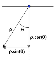
Figure 2.
Polar coordinates {ρ,θ,φ}
The azimuth angle φ denoting a rotation around the axis (dotted line) is not shown.
The solution: gravitoids and gravidomes
In order to find the solution we will
(a) assume a generic contour curve,
(b) calculate the volume V of the corresponding body,
(c) calculate the gravity G at the barypole B, and
(d) find the equation for r(θ) which makes G stationary under the constraint of constant V.
Detailed workout of each point:
(a) Let r(θ) be continuous in [0,π/2] and possess a derivative anywhere in (0,π/2).
(b) In the polar coordinates {ρ,θ,φ} shown in Figure 2, an infinitesimal volume element is
(1)  . .
For the volume V we therefore have
(2)  . .
(c) The calculation of the gravity vector Q at point B is simplified by the symmetry which tells us that Q is parallel to the axis. We therefore need to sum up just the parallel components due to all the masses present in the volume elements dV. Since the density η is constant, the mass present in dV is ηdV which, according to Newton's law, contributes to Q by an element dQ whose magnitude is |dQ| = G(ηdV)/ρ2, where G is the gravitation constant. Since the projection of dQ onto the axis is dQ = |dQ| cosθ, the formula for Q = |Q| becomes
(3)  . .
|
|
When my grand-grand-daddy says gravity, what he means is the intensity of the gravitational field which is defined as the force it exerts on a unit mass (this is in line, for example, with the intensity of electric field defined as the force it exerts on a unit charge). The SI dimension of Q is therefore that of [force/mass]=[acceleration]=[m/s2]. The mean gravity on the Earth surface is 1 g = 9.80665 m/s2 (click here for the values of physics constants).
|
|
(d) Applying the tools of variational calculus, assume that r(θ) is subject to an infinitesimal functional variation δ(θ).
This leads to the following variations of V and Q:
(4)  . .
The first of these equations exploits the calculus of derivatives according to which the variation in r3(θ) equals 3r2(θ)δ(θ).
In practice, we need to consider only those variations δ(θ) which leave the volume constant, i.e., for which δV = 0. Under this constraint, we would like Q to be extreme which means that we should have also δQ = 0 for any admissible δ(θ).
One of the basic approaches of variational calculus is to form the linear combination (δV + λ δQ) and see whether there exists a constant value of the Lagrange multiplier λ for which the combination is null regardless of δ(θ). If we are lucky and such a constant value exists then satisfying the constraint δV = 0 implies that the desired condition δQ = 0 is valid as well. In our case
(5)  . .
which is zero regardless of δ(θ) if and only if
(6)  . .
Consequently, λ is constant if and only if r2(θ) is proportional to cos(θ), which is the condition defining the optimal contour curve. We will write
(7)  . .
with D being the value of r(0), i.e. the distance between the barypole B and the opposite contour point A which we will call antipole. Figure 3 shows the normalized optimal contour curve for D = 1. In what follows, we will call gravitoid the optimal contour curve and gravidome the body obtained by its rotation around the axis.
Once the constancy of λ is guaranteed, its actual value becomes irrelevant. What interests us more is the relationship between D and the gravidome volume V, as well as its barypole gravity Q. Substituting (7) into (2) and (3) and evaluating the elementary integrals, one obtains
(8)  . .
The shapes of a gravitoid curve and of a gravidome body are therefore fully defined by a single parameter (such as the depth D or the volume V). All such shapes are similar and can be obtained by simple scaling with respect to the barypole of the normalized shape curve. In this sense, Figure 3 represents all of them.
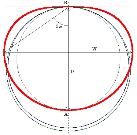
Figure 3. A gravitoid (cross section of a gravidome).
The drawing shows the gravitoid curve (bold red) with its barypole B and antipole A. The corresponding gravidome is formed by rotating the gravitoid around the axis AB. Also shown are the depth D and the width W of the two objects and the gravidome's insribed sphere (gray, smallest), equivalent volume sphere (blue, intermediate) and equivalent gravity sphere (green, largest).
Gravidome numerology
Equations (8) link together the gravidome volume V, its barypole gravity Q and its depth D, leaving independent just one of them. Figure 3 shows also the gravidome width W whose numeric value can be determined as follows.
Using Figure 2 and Eq.(7), we see that the width w(θ) corresponding to polar angle θ equals
(9)  . .
Finding the polar angle θ which maximizes the latter ratio and the corresponding maximum value of W/D is elementary.
It turns out that
(10)  (see OEIS A208745). (see OEIS A208745).
making the gravidome about 24% wider than it is deep.
|
|
Through subsequent decades much fuss has been made about the fact that the polar angle corresponding to the maximum width is equal to the so-called magic angle (about 54.73561... degrees) whose cosine is the root of the second-degree Lagrange polynomial. Likewise, some find magic in the fact that the ratio W/2D differs by mere 0.38% from the golden ratio related (among other things) to Fibonacci numbers. Though I consider such speculations mildly foolish, the recognized relation between the golden ratio and human esthetic cannons might explain the fact that most people find the shapes of gravitoids and gravidomes very pleasing.
People also immediately noticed the similarity between the gravidome shape and that of the original variety of tomatos. This is why Ad Astra competitors initially used to call gravidomes tomatoids, accompanying the mentions with [stupid] sneers and an assortment of derogatory accents.
|
|
From Eqs.(8) it is easy to see that the volume of a gravidome is exactly 8/5 that of its inscribed sphere with diameter D. Vice versa, the diameter of a sphere with the same volume as the gravidome (the V-equivalent sphere) equals D multiplied by the cubic root of 8/5 (about 1.1696).
From the space engineering point of view, a more interesting question is the diameter and volume of the G-equivalent sphere - one which has the same surface gravity as that at the barypole of a gravidome. We know that the gravity outside a sphere (including its surface) is the same as though all the mass were concentrated in its center. The surface gravity of a sphere of diameter d filled with a material of density η therefore equals to
(11)  . .
Comparing this with Eqs.(8), the diameter d of the G-equivalent sphere is (6/5)D and the ratio of its volume to that of the gravidome equals (27/25) = 1.08. In other words, using a gravidome instead of a sphere to produce a certain gravity, the required mass is 8% less. One can also reverse the question: Given a fixed amount of material, how much greater will be the gravity if I shape it as a gravidome rather than as a sphere? The answer is 2.6 % (the cubic root of 1.08).
|
|
Around this point the margins of my grand-grand-daddy's notes are densely covered with vulgar comments definitely not fit to be repeated in print. He evidently hoped for more substantial mass savings and was disillusioned by the 8% which he thought unworthy of the trouble. Little did he know about how requested and expensive would inertial mass become in the future. The cost of any gravity engineering project is strictly proportional to the mass it manipulates (we talk about D's in the hundreds of kilometers). Since the net profits of gravity engineering Companies rarely exceed 10%, you can imagine what an impact a cost reduction of 8% can have. Which is part - though not all - of the reasons behind the success story of Ad Astra.
Personally, I find more puzzling the theological aspects of the problem. Why is it that the optimal solution (the gravidome) differs from the intuitively most perfect solution (the sphere), even though the difference is so small? Does this not diminish the Glory of His Creation? I hope not.
Gravinions
What really propelled Ad Astra ahead of its competitors was not the gravidome concept as such but the developments which arose from giving a second look at the equations for Q in (8) and (11). My grand-grand-daddy jotted the essential comments on half a dozen of paper napkins, some of which stained by spaghetti sauce (pomodoro con basilico). This is what I have managed to save.
|
|
From Eqs.(8) and (11) it follows that, regardless of the shape of an object, the gravity Q on its surface is directly proportional to the density η and to the object's linear dimension (D or d). Now assume that somebody offers you a material whose density is twice as high as the density of the stuff you are currently using. This will enable you to produce the same gravity as before with gravidomes (or spheres, if you prefer them) scaled down by a factor of 2 and thus reduce their volume by a factor of 8. Consequently, their mass will be reduced by a factor of 4 (2 times denser material in 8 times smaller volume).
|
|
This consideration explains a lot about the most basic rules of gravity engineering. Give me a material twice as dense as what I currently have and my costs will drop to one quarter! The catch is that, in actual life, your costs drop much less since the price of inertial mass has become almost exactly proportional to the square of its density. Hence the frenetic search for exceptionally dense materials. To find a large unclaimed dense object anywhere in the Solar system is today a front-page event and most governments are funding research aiming at the production of the hypothetical ultra-atoms with gigantic nuclides which, according to some eccentric theoreticians, might be stable.
|
|
Considering this, plus the fact that raw matter is always heterogeneous, it is likely that sorting its components according to their density might help. For example, consider a comet with mass M half of which is ice (density ηice = 1) and half rock (ηrock = 5). That amounts to an ice volume of Vice = M/2, a rock volume of Vrock = M/10, and a total volume of Vtotal = 6M/10 so that, when unsorted, the comet has an average density of ηtotal = 10/6. Suppose now that we sort the material and construct a gravidome only from the recovered rock Then, according to the last of Eqs.(8), the ratio between the barypole gravity of the rock-only gravidome and that of the gravidome build from the unsorted stuff is
(12)  . .
This is a huge success, since we are getting 65% more gravity using only half of the comet !!! Vice versa, if we insisted on getting the same boost in gravity just by adding more unsorted comet matter, we would need a total of 4.5 comets ! The trick clearly consists in the fact that the denser the matter, the more mass can be located close to the barypole.
|
|
Well, this is why density sorting became a buzz word in gravity engineering as soon as the discipline was established as a distinct branch of space engineering. You pick up any of their numerous Magazines and it is full of ads for asteroid-size mass sorters of all kinds.
|
|
So what if we used all the matter we have, but sorted it first into classes with different densities. The question is: how do we arrange the various lots within the novel, heterogeneous gravitational attractor? Surprisingly, this is an easy problem which can be solved by plain inspection with no math at all.
Consider first just the two outer components A and B in Figure 4 (ignoring C and D). The two nested bodies A and B are gravidomes which share a common barypole and a common rotation axis. The inner barydome is made of the higher density material while the lower density material fills the space between the barydomes.
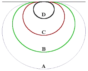
Figure 4. A four-component gravinion.
A gravinion consists of a number of gravidomes nested as shown. The density of the materials increases from the outermost gravidome towards the innermost one.When raw mass (debris, asteroid rock and ice, etc.) is sorted according to its density, melted and arranged into a gravinion, the resulting gravity at the barypole is much higher than using unsorted mass.
To understand that this is really the best arrangement, consider first a single barydome A having a homogeneous density ηA (the smaller of the two). We know that, for A by itself, a barydome is the optimal solution with the highest possible barypole gravity. Now imagine that we introduce inside barydome A a body with the higher density ηB. Rather than replacing part of the barydome A volume, however, we will think about it as if we were superposing a body whose density equals the difference ηB-ηA (since gravity forces are additive, this does not alter them in any way). Now all we need to do is to optimize the location and the shape of a body with the difference density located inside A but otherwise quite independent of it. The solution to this second problem is of course again a gravidome with the same barypole. To complete the solution, one just needs to adjust the sizes of the gravidomes so as to make sure that the volume of the inner one matches that of the available denser material, and the difference of the two gravidome volumes equals the volume of the lighter material.
Using recursion, the solution is easily extended to multi-component situations. Suppose that we have n components, each with a density ηk and volume Vk, and assume that, without lack of generality, η1 > η2 > ... > ηn. The solution is a series of nested gravidomes with depths D1 < D2 < ... < Dn < defined by
(13)  . .
The gravity at the barypole is then
(14)  . .
and it is always greater than the maximum barypole gravity achievable when using a homogeneous mixture of the components.
|
|
My grand-grand-daddy shows the multi-component solution but does not attribute any name to the objects (he did not appreciate them much, anyway). Decades later, Ad Astra introduced them commercially under the name gravinions which was a contraction of 'gravidome' and 'union'. Again, our competitor's agents spread around the somewhat derogatory term 'onions' which, I regret to say, stuck and became widespread (as in 'what a nice little onion you have here').
Through the years, of course, much more math, both basic and applied, has been dedicated to gravidomes (just the number of dedicated monographs exceeds a thousand). In future I will return to some of their most popular aspects so, please, return back to this Library to see whether something new has been added.
Abdul Aziz Sykora ibn Enrico ibn Martino ibn Stan,
4th of July, 2123 years after the death of Prophet Christ.
|
|
References
MATH:
- Giaquinta Mariano, Hildebrandt Stefan,
Calculus of Variations I: The Lagrangian Formalism,
Springer Verlag 2006. ISBN 978-3540506256.
more >>
- Giaquinta M., Hildebrandt S.,
Calculus of Variations II: The Hamiltonian Formalism,
Springer Verlag 2006. ISBN 978-3540579618.
more >>
- Dacorogna Bernard,
Introduction To The Calculus Of Variations,
Imperial College Press 2004. ISBN 978-1860945083.
more >>
- Kumar Naveen,
An Elementary Course of Variational Problems in Calculus,
Alpha Science International 2004. ISBN 978-1842651957.
more >>
- Moiseiwitsch B.L.,
Variational Principles,
Dover Publications 2004. ISBN 978-0486438177.
more >>
- Smith Donald R.,
Variational Methods in Optimization,
Dover Publications 1998. ISBN 978-0486404554.
more >>
- Sagan Hans,
Introduction to the Calculus of Variations,
Dover Publications 1992. ISBN 978-0486673660.
more >>
- Fox Charles,
An Introduction to the Calculus of Variations,
Dover Publications 1987. ISBN 978-0486654997.
more >>
- Weinstock Robert,
Calculus of Variations,
Dover Publications 1974. ISBN 978-0486630694.
more >>
Added on 2 March 2012:
- Rockafellar R.Tyrrell,
Variational Analysis,
Springer 2011. ISBN 978-3540627722.
more >>
- Dacorogna Bernard,
Direct Methods in the Calculus of Variations,
Springer 2010. ISBN 978-1441922595.
more >>
GRAVITY ENGINEERING:
- Web link to this page (this is cyclic reasoning in practice)
- A page on Space Future which is a nice entry gate to the topic: Who is Who - Theodore Hall
- Hall T.W., The Architecture of Artificial-Gravity Environments for Long-Duration Space Habitation,
Doctoral dissertation, University of Michigan (Architecture Dept.) 1994.
- Hall T.W., The Architecture of Artificial Gravity: Archetypes and Transformations of Terrestrial Design,
pages 198-209 in Space Manufacturing 9: The High Frontier - Accession, Development and Utilization,
SSI 1993 Proceedings, Editor Faughnan B., American Institute of Aeronautics and Astronautics.
- Kim K., Spelke E.S., Infants' Sensitivity to Effects of Gravity on Visible Object Motion,
Journal of Experimental Psychology: Human Perception and Performance 18, 385-393, 1992.
- Hall T.W., The Architecture of Artificial Gravity:
Mathematical Musings on Designing for Life and Motion in a Centripetally Accelerated Environment,
pages 177-186 in Space Manufacturing 8: The High Frontier - Energy and Materials from Space,
SSI 1991 Proceedings, Editor Faughnan B. & Maryniak G., American Institute of Aeronautics and Astronautics.
- Connors M.M., Harrison A.A., Akins F.R., Living Aloft: Human Requirements for Extended Spaceflight,
NASA Scientific and Technical Information Branch, Special Publication 483, 1985.
- Oberg J.E., Oberg A.R., Pioneering Space: Living on the Next Frontier,
McGraw-Hill 1986.
- Johnson R.D., Holbrow C., Editors, Space Settlements: A Design Study,
NASA Scientific and Technical Information Office, Special Publication 413, 1977
- O'Neill G.K., The Colonization of Space,
Physics Today 27/9, 32-40, 1974.
- Payne F.A., Work and Living Space Requirements for Manned Space Stations,
Proceedings of the Manned Space Stations Symposium, April 20-22, 1960.
Modifications done on 2 March 2012:
- The gravitoid constant W/D of Eq.10 became part of the On-Line Encyclopedia of Integer Sequences as #A208745.
Consequently, an appropriate link was added.
- References were enhanced with correct ISBN numbers, and two more were added.
- Graphic was slightly improved by suppressing image artifacts.
|
|