Introduction

When discussing NMR sensitivity, people often over-concentrate on the nominator of the S/N ratio, discussing the dependence of NMR signal intensity on all kinds of parameters such as the operating (Larmor) frequency, sample/coil temperature, coil Q-factor, sample/coil filling factor, etc. Unfortunately, signal intensity, by itself, is irrelevant because amplifying any electric signal by any desired factor is a trivial task. When it comes to a S/N ratio, the noise in the denominator is just as important as the signal and it, too, has its own dependencies on frequency, temperature, etc.

Consider, for example, the S/N dependence on operating frequency. For a given nuclide, the operating frequency f is proportional to the applied magnetic field B (the proportionality constant being the nuclide's gyromagnetic ratio). The signal intensity S is proportional to the equilibrium nuclear magnetization [1] in the field B which, to a good approximation, is proportional to B and therefore also to f:

(1)   ,
where M is the nuclear magnetization of the sample, ρ is the volume density of the measured nuclides (ρ=N/V), γ and S are their respective gyro-magnetic ratio and spin, h and k are respectively the Planck and Boltzmann constants [2], T is the absolute sample temperature, B is the magnetic flux density and f is the Larmor frequency of the nuclides in the field B.

When using an inductive sensor such as a pick-up coil, one must also consider the fact that the picked-up signal is proportional to the derivative of the precessing transversal component of nuclear magnetization rather than to the component itself. This brings in another factor of f and thus leads to the textbook statement according to which NMR signals are proportional to the square of f.

In the past, people used to jump from this to the simplistic conclusion that NMR sensitivity, measured by means of the S/N ratio, was also proportional to f-squared. This is one of the clichés which, today, start showing wide-open cracks.

A factor which greatly contributed to the f-squared myth was the almost ubiquitous use of induction coils as NMR sensors, combined with the fact that these are nearly always incorporated into a tuned circuit with a matched impedance R. The value of R then dominates the device's thermal noise, whose mean power density is given [3] by the Johnson formula.

(2)   
where G(f) is the power density of the electric noise with respect to frequency f, k is Boltzmann constant [2], T is the absolute temperature of the circuit and R is the ohmic part of its impedance. The low-frequency approximation is valid when hf/kT<<1 which, at room temperature, implies f << 6200 GHz, a condition which is in NMR always satisfied. The index t stands for thermal and n is the rms noise voltage amplitude associated with a bandwidth Δf within the low-frequency approximation.

Notice that R (typically 50 Ohm) is usually chosen in a somewhat arbitrary way on the basis of commercial availability of coaxial cables with matching impedance, rather than on physical considerations regarding the thermal noise of the sensor. Reducing the matched impedance R may be another avenue towards S/N ratio optimization.

The use of induction coils still persists across almost the whole range of operating frequencies. Exceptions are resonant cavities which are becoming feasible for protons at the highest available fields and superconducting quantum interference devices (SQUIDs) which are, unfortunately, are most effective at very low fields (down to zero but, at present, less than about 0.12 T). For actual inductive pick-up coils the signal induced by a given oscillating magnetic moment is only approximately proportional to f, but nevertheless essentially correct. It is also present in resonant cavities, even though deviations from linearity are in this case more marked. On the other hand, it is absent in SQUID detectors whose sensitivity exceeds that of inductive coils by many orders of magnitude!

In principle, one could try and use a number of field-dependent phenomena to detect the NMR signal. Magneto-resistivity and various magneto-optical properties of many special materials come to mind in this context and there is a lot of research going on in that direction, propelled by the development magnetic data-storage devices. In particular, field-dependent optical transitions with their extremely fast response times and their conceptual capability of converting field variations into frequency modulation might yet lead to a complete revolution in NMR spectroscopy.

Back in 1946, Bloch and Purcell chose inductive pick-up coils simply because they were then the simplest oscillating-magnetic-field sensors to think about. It is amazing that they maintained the status of best such detectors for so many decades afterwards! However, times might come when the ubiquitous "coil" will be more obsolete than a stone ax.

At present, NMR branches which have no use for chemical shifts (such as simple MRI) start timidly looking towards SQUIDS. As detectors, SQUIDS are still rather unwieldy but, given their rapid development, I would not be surprised if, within a generation or so, most clinical MRI were done with SQUIDs in very weak magnetic fields (such as the Earth field). The same might apply also to the presently over-neglected wide-line NMR spectroscopy of solids in which field-independent dipolar interactions mask out the field-dependent chemical shift terms of the spin Hamiltonian. However, since this article is not about SQUIDS, and since NMR spectroscopy will always need high magnetic fields in order to spread-out the chemical shifts, let us return to our classical S/N ratio.

Given the uncertainty about what the noise term in the denominator should/could be, a theoretical physicist is likely to try and invoke first principles in order to estimate the ideal electromagnetic noise originating, like the NMR signal itself, within the sample.

Everybody knows that, at thermal equilibrium, the random electromagnetic radiation emerging from any physical system, given by the Planck's black-body radiation formula, has the mean frequency-distribution density

(3)   
where E(f) is the power density of the radiation with respect to the frequency f emitted into a subtended solid angle of 1 sr, T is the absolute temperature of the radiating body, and h and k are again the Planck and Boltzmann constants (2). The low-frequency approximation is again valid when hf/kT<<1 which, at room temperature, implies f << 6200 GHz.

According to Eq.(3), a thermal noise power of a sample is proportional to f-squared or, equivalently, its rms noise amplitude is proportional to f. Consequently, taking into account Eq.(1) and using a detector which has no inherent frequency dependence, S/N ratio should not depend upon the operating frequency. The same result, however, is obtained even when using an inductive pick-up coil, due to the fact that such a detector applies the extra f factor both to the signal and to the noise.

Since physical theory is the ultimate limit, we conclude that, contrary to most textbooks and to many false but well-rooted beliefs, the theoretical maximum S/N ratio is independent of f. Quantitative estimates of its value present quite a few tricky problems and apparently can't be done without some assumption about the detector type (I will return to this problem at a later occasion). Nevertheless, they all indicate that, in actual practice, we are off by orders of magnitude!

To sum up the current situation, the NMR signal is what it should be according to physical theory, while the noise is not so by a long shot and appears to be totally determined by current [inadequate] technology with almost no part of it being due to the thermal noise within the sample.

This, in a sense, is both bad news and good news. The bad news is that when it comes to detecting NMR signals, we are presently doing an extremely lousy job. If only we were more capable, we could do in one scan what we can't nowadays achieve in a month of data accumulation. The good news is that there is an enormous room for improvement. Personally, I prefer to concentrate on the second aspect rather than shedding tears on the first one.

Conventional NMR detector

The customary answer of an electronic engineer to the question "what is an NMR detector" usually includes the receiver channel, typically composed of a preamplifier, an inter-frequency mixer (when IF is used), a down-converter (improperly called phase detector) with two quadrature outputs, a dual set of low-frequency filters, and an analog-to-digital converter (ADC). Novel digital receiver designs contain essentially the same parts, except for the fact that the analog-to-digital conversion is done at an earlier stage (in some cases immediately after the preamp) and the subsequent tasks are carried through mathematical operations on the digitized data. The only conceptual difference is that one needs to insert suitable decimation filters in front of the final audio-filters in order to accommodate the extremely large ratio between the input and output bandwidths.

From a physicist's point of view, such a description needs to be completed by including the actual oscillating-magnetization sensor, typically an inductive pick-up coil inserted into a passive network and matched to a connecting coaxial cable of some characteristic impedance. The sensor permits to detect the precessing nuclear magnetic dipoles and transfer part of their energy to the preamplifier. The diagram of the complete system looks like this:

Figure 1. Block diagram of an NMR detector & receiver channel

The spin system, located inside the coil L, is first excited by a brief RF pulse from the gated transmitter Tx. The subsequent transient NMR signal induces an oscillating emf in the coil L which, together with the tuning (red) and matching (green) capacitors makes part of a resonant circuit, matched to an effective impedance Z (usually 50 Ω). The signal S is then carried by a coaxial cable to the transmitter/receiver separator TRS whose task it is to isolate the preamplifier from the transmitter during the RF pulse. This may be just a λ/4 coaxial cable with crossed-pairs of switching diodes as the one shown in the inset on the right, or a more sophisticated 90° phase-shift circuit. The signal then reaches the preamplifier from which it proceeds to the receiver proper. Should inter-frequency (IF) be used, the first receiver block would be an IF mixer with suitable input and output filters, but since that would not affect the present discussion, we have omitted it and assume direct detection. The receiver consists of a dual down-converter DCV using two reference-frequency inputs in quadrature, followed by two low-pass filters which extract the desired low-frequency signals U and V. The Figure does not show the analog-to-digital converter(s) (ADC's) which, in traditional analog receivers, would be located at the very end. In modern digital receivers, the sampling is done at an earlier stage (in the case of direct sampling, even right after the preamp). Red color indicates radio-frequency (RF) paths, with dual lines standing for coaxial cables. Blue color indicates low-frequency paths (be they analog cables or digital busses).

For the purposses of this paper, we will adopt the following terminology: 
- Sensor, or probe, includes the coil and its matching circuitry.
- Preamplifier includes the very first amplification stages but no frequency-changing elements.
- Front-end includes the probe, the transmitter/receiver separator TRS and the preamplifier.
- Receiver includes the receiver proper, any IF filters and mixers when IF is used, and the ADC'c.
- Detector is the whole assembly including all the units listed above.

Figure 1 shows also the principal noise sources involved in an NMR detector:

 Sensor noise n_s

This includes the thermal noise from the probe given by Eq.(2) as well as any anomalous noises which might be picked up by the probe (brought-in, for example, by the thermocouple of a temperature regulation device), reach the separator circuit from the transmitter or be generated within the separator circuitry. In the following we will consider such anomalous noises to be absent even though, in practice, it may be far from easy to get rid of them.
It is very important to understand, however, that as long as the probe is tuned and matched to an impedance R, its thermal noise is determined exclusively by R and has nothing to do with the nature or the amount of the sample, much less with its spin sub-system.

Equivalent input noise of the preamplifier, n_p 

Every electronic device, active or passive, gives rise to a noise contribution of its own. Normally, this is approximately proportional to the device gain so that it is convenient to think of it as though there were a noise source of constant mean amplitude connected to the device input, a quantity known as the equivalent input noise. Since, like the Johnson noise, it is closely linked to the spectral density of the noise power, the rms amplitude of the equivalent input noise is proportional to the square-root of the considered bandwidth and specified in nV/√Hz. Unlike Johnson noise, the equivalent input noise of active electronic devices often exhibits a strong frequency dependence, a fact which strongly affects the actual S/N ratios.

Equivalent input noise of the receiver, n_r 

As any other physical component, the receiver has its own equivalent input noise. The situation is somewhat different in digital receivers with direct sampling (i.e., analog-to-digital conversion of the signal even before the down-converter) where much of the receiver noise arises from sampling jitter and from ADC rounding errors, both of which have a very characteristic frequency dependence. Another non-standard contribution is due to the phase noise of the reference signals.

The sensor signal and the sensor and equivalent preamp noises, before summing up with the receiver noise, get a a boost from the preamplifier gain A (typically 10-1000) and thereafter also from the receiver gain G (variable). The equivalent receiver noise, of course, gets only amplified by the factor G. Since mutually uncorrelated random noises have additive variances rather than amplitudes, the total signal S and noise n amplitudes at the output of the receiver are given by

(4)   

with S_s being the sensor signal. The final S/N ratio can be therefore written as

(5)   

Statistically speaking, the three noise sources are often roughly comparable in size. It follows that when A is large, the effect of the receiver noise is much smaller than that of the combined sensor and preamp noises for which we shall use the term front-end noise. For good-quality receivers, especially the digital ones, the final S/N ratio is virtually the same as that at the output of the preamplifier.

When it comes to mutually incoherent noises, their additive property is the variance (or, equivalently, power). Consequently, when several noise sources are present, one of them tends to dominate. For example, if noise amplitudes of two sources A and B have a ratio of 1:4, the relative impact of source B on the combined noise is only about 1:16. Hence comes the master principle of electronic engineering: always cure first the part which hurts most.

Unfortunately, the part which hurts most on modern NMR and MRI instruments is not always the same. On some it is the probe, while on others it is the preamplifier (it should never be the receiver, but one can't be sure even of that).

Note: There are simple ways of assessing the contributions of the three different noise sources and making sure that the receiver does not degrade the S/N ratio. They consist in shorting selected combinations of RF paths and/or replacing them by passive resistors. However, a universal recipe for how to do it might be dangerous since instrument manufacturers sometimes use the coaxial paths to distribute DC power as well as RF signals.

Reducing the probehead noise

In the case when the dominant noise contribution arises in the probe, one can try to reduce it by modifying the pertinent parameters of the probe electronics.

One method consists is tuning and matching the probe circuits to a sub-standard impedance. According to Eq.(2), this will reduce its thermal noise but it will also complicate the coupling between the probe and other RF units in the system. Nevertheless, it is a valid possibility to keep in mind and we shall return to it later.

Another approach consists in reducing the thermal noise of the probe by cooling its circuits. For example, when a network is cooled down from room temperature to liquid helium, its thermal noise power drops (theoretically) by a factor of about 70, amounting to factor of 8.4 in terms of S/N ratio.

Naturally, cooling the probe circuitry while keeping the sample at normal temperature presents a considerable technological challenge. Moreover the gain is always only partial. In a tuned and matched probe circuit, the effective ohmic impedance can be tracked to three energy-loss pathways: ohmic dissipation in the coil, dielectric losses in the capacitors and dielectric losses in the sample. Freezing the tuning capacitors might make them unusable, and one certainly does not wish to freeze the sample. This leaves only the fixed capacitors and the coil, whose contribution to the circuit noise may, but need not, be dominant. In general, cooling the coil works well in some cases, especially in the small-volume probes common in NMR spectroscopy where loading of the circuit by the sample is negligible, and it is worth trying, but it is not a universal panacea.

Cooling the preamplifier

When the dominant noise contribution arises in the preamplifier, one can try to cool the latter. The equivalent input noise of a preamp often has a marked temperature dependence (since active silicon is involved, the dependence may be exponential). Consequently, cooling it even by a relatively modest amount might improve its noise characteristics quite a lot.

With decreasing preamplifier temperature, however, the values of its internal components drift and so do the working points of its transistors. Consequently, the device might at some point start loosing gain, a fact which could well make the drop in noise useless. In general, preamplifiers cooled down to really low temperatures (liquid nitrogen or helium) need to be specially designed to work in such an environments.

Preamplifier clusters

Another way of improving the noise performance of a preamplifier consists in connecting N>1 identical preamps in parallel and summing their outputs. The gain of the combined device is then equal to NA but, since the equivalent input noises of the individual devices are uncorrelated, their sum is a random noise whose variance is greater than that of each of the devices by the square-root of N. These two factors have the same effect as if the equivalent input noise of the preamp were reduced by square-root of N.

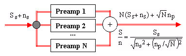
Figure 2. Block diagram of a preamplifier cluster

A problem which needs to be addressed with care is the realization of the input matching/splitting. For example, an RF splitter in place of the black dot would not do since, even in the ideal case, it would cut the sensor signal and sensor noise amplitudes by square-root of N and thus leave the final S/N unchanged.

There is one more potential advantage in using preamplifier clusters. All NMR transmitter-receiver separation/protection schemes include a pair of crossed diodes at the input of the preamplifier. Diodes, however, are semiconductor components with a noise of their own. In a preamplifier cluster, it is both possible and advisable to use only one crossed-diodes node for the whole cluster instead of having one in each preamp (this is why all the crossed diodes in Figure 1 were considered as part of the TRS circuit). The result is an additional reduction of the equivalent input noise of the preamplifier cluster.

The practical realization of the preamplifier cluster idea is somewhat more complicated because of the matching requirements involved. If each of the individual devices has an input impedance Z than the combined device has the input impedance Z/N and a similar argument applies to the output.

The output matching is not a problem since, as already explained, a minor addition of noise from an extra circuitry after the preamp does not appreciably deteriorate the S/N ratio. One can therefore use a simple RF combiner (especially considering that the effect of combiners on S/N ratios is anyway only marginal). An even more perfect solution consists in direct digital sampling of each preamp output and digital summing/averaging of the data. This would, in addition, also reduces the round-off errors of the digitizers.

The input matching is more tricky since, as can be easily shown, RF splitters worsen the S/N ratio. One way is to use preamplifiers whose input impedances are larger than that of the rest of the circuitry. For example, connecting in parallel six preamplifiers with input impedance of 300 Ω (an industry standards), one ends up with a preamp cluster whose input impedance is 50 Ω (another industry standard). Since many preamplifier transistors attain minimum noise figure for input impedances larger than 50 Ω, this approach is quite viable.

An even better way consists in using N preamplifiers with standard input impedances Z and matching the probe to Z/N (an example for N = 2 is shown below). This has the additional advantage of decreasing the sensor noise by square-root of N and thus assuring, at least theoretically, a square-root of N improvement of the S/N ratio regardless of whether the preamp noise is dominant or not. In practice, there is a limit to matching a probe to an excessively small impedance, a fact which limits the value of N (though values from 2 to 8 should be acceptable). Another complication arises from the fact that the transmitter output also needs to be matched to the low Z/N impedance of the probe. This can be done either by re-desining or re-tuning the final stage of the power amplifier, or by means of an external impedance-changing RF transformer (the slight power loss associated with such a device is normally quite tolerable).

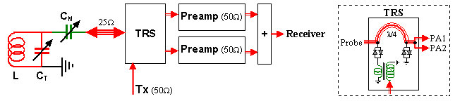
Figure 3. Example of an NMR front-end system with two preamplifiers and a 25 Ω probe.

Triple red lines indicate 25 Ω coaxial cables (or two parallel 50 Ω cables). The box on the right is an example of the internal wiring of a transmitter/receiver separator with its 90° phase shifter (in this case just a λ/4 coaxial cable), but including also the transmitter impedance-matching transformer and the switching RF diodes. The block labeled "+" can be realized using a simple RF combiner.

Multiple detectors

When the object of a measurement is itself the dominant source of measurement errors, the only thing one can do, when possible and when the errors distribution probability function satisfies certain conditions, is to repeat the measurements and average the results. In NMR, this corresponds to the widespread practice of averaging the transient signals generated in successive cycles of relaxation-excitation-detection.

A somewhat different situation arises when the dominant source of measurement errors is the measuring device (detector). In such a case there is an additional possibility consisting in using a number of detectors in parallel and averaging their outcomes.

There is nothing surprising about this. As far back as Old Egypt, if not earlier, when a piece of land was changing hands, it was a common practice to ask several surveyors to estimate its size and average the individual outcomes. Likewise, an insect's composite eye is nothing but a cluster of imperfect sensors which together amount to a much better one. The approach is universally applicable, provided that the interaction between the measurement device and the measured system is small enough not to change the system's properties.

In NMR, the condition of negligible interference between the spin system and the detection hardware appears to be guaranteed by many orders of magnitude. There is therefore little doubt that NMR S/N ratios can be improved by applying multiple detectors and summing/averaging their outputs. Two detectors imply an improvement factor of √2, four detectors a factor of 2, etc.

Dual coil probeheads

As anticipated above, when a sensor is noisy and weakly coupled to the observed system, the composite eye principle should work. In the case of NMR spectroscopy, this implies, first of all, winding two or more pick-up coils around the sample - a task which is delicate but not impossible (Figure 4). It is mechanically convenient to wind the coils in a manner to make them orthogonal, an arrangement which turns out to be desirable also for other reasons to be discussed later.

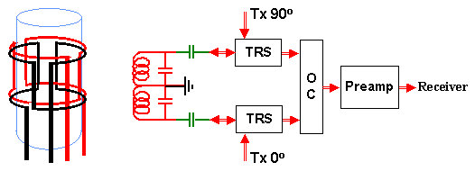
Figure 4. Block diagram of a simple dual-coil NMR detection system

On the left is a schematic drawing of two orthogonal saddle coils wound around a sample tube (we assume axial arrangement with the main magnetic field parallel to the sample tube axis). The circuit diagram on the right shows two transmitter/receiver separators with two orthogonal transmitter inputs. The two induced signals are in this example combined using a passive orthogonal RF combiner OC. This is admissible because good quality RF combiners (unlike splitters) have only marginal adverse effect on S/N ratios.

The two orthogonal transmitter inputs in Figure 4 could come either from two distinct power amplifiers or, more simply, could be derived from the same power amplifier by means of an orthogonal RF power splitter. This would actually enhance the intensity of the RF field in the coil (and, consequently, reduce the 90° pulse width) because the orthogonal excitation arrangement generates a rotating RF field which is twice as effective as an oscillating one generated by a single coil.

Regarding the S/N ratio, the important fact is that the thermal noises arising from the two coils are not mutually correlated. This property is sometimes linked with the fact that the two coils are electrically orthogonal. In practice, the orthogonality is usually not essential for the two noises to be un-correlated since, as discussed above, much of the sensor noise is generated right in its circuitry rather than being picked-up from the sample. However, the orthogonal arrangement guarantees the statistical independence of the two noises regardless of where they come from.

When two separate induction coils are available, it is particularly easy to combine them with two separate preamplifiers as shown in Figure 5.

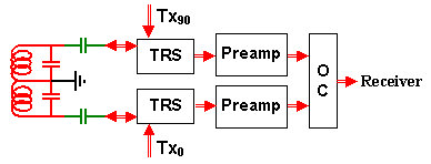
Figure 5. Dual-coil NMR detection system with two preamplifiers

This arrangement guarantees a sensitivity gain of square-root of 2 regardless of whether the dominant noise source is the sensor or the preamplifier. In addition, any doubt about the noise quality of the orthogonal coupler is removed since it's relative noise contribution, should there be any, gets divided by the preamplifier gain.

A word of caution: do not commit the error of concluding that the arrangement of Figure 5 improves the S/N ratio by a factor of 2 (square-root of 2 due to the two coils and another square-root of 2 due to the two preamps). In reality, it is the sum of the source and preamp noises whose combined effect gets suppressed by a single square-root of 2 factor. The advantage of Figure 5 arrangement is that it helps always, while that of Figure 4 helps only if the dominant noise source is n_s.

Complete chiral detectors

We can now return to the question of the receiver unit and its own noise which, so far, we have decided to neglect. The ideal thing would be to double also the receiver units and use two complete receiver channels. That, at least, would eliminate any discussion about whether the receiver noise is really ineffective or not. We are therefore back to replicating the whole receiver rack, a thing I have so far discouraged you from doing.

The fact is that using old-fashioned analog circuitry, a complete receiver unit represented quite a lot of circuitry and replicating it could have been quite costly. With the advent of digital receivers, however, the situation has changed dramatically. A single FPGA chip such as Xilinx's Virtex II or Altera's Stratix II can easily accommodate up to four complete digital receivers in a single chip so that replicating receivers during a new design is as simple as a pair of copy and paste clicks and costs absolutely nothing. Even the few extra ADC converters in front of each receiver are nowadays quite affordable (for example, the Analog Devices AD9430 chip goes up to 210 Msamples/s and costs less than a family dinner at a restaurant). Hence not to replicate digital receivers would be much less then intelligent.

When IF is used, one must replicate also the old-time, analog IF mixers, including the anti-aliasing band-pass filters which precede them and the output-band filters which follow them. This will push future developments towards direct detection, even at the cost of having to resort to under-sampling. Since the presence or absence of IF anyway does not affect our S/N discussion, we shall continue to ignore it.

Again, duplicating the whole detection hardware, by itself, does not increase S/N ratio by a factor larger than the usual square-root of 2 - it just makes sure that, no matter what, the gain will really occur.

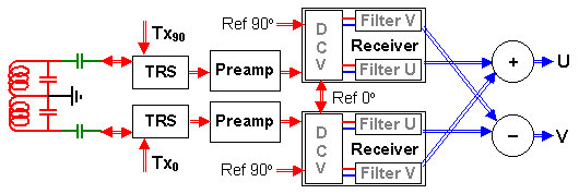
Figure 6. Complete dual-coil, dual-receiver chiral detector

Notice that the receivers share the two orthogonal reference frequency signals. Their respective outputs, however, are shifted by 90° because of the fact that the coils are orthogonal. At the audio level, the digital output busses U and V of both receivers must be added and subtracted as shown in order to obtain the final in-phase (U) and out-of-phase (V) signals. In a direct-detection, direct-sampling digital version of the device, the ADC's should be part of the receiver input circuitry or, equivalently, of the preamplifier output (digital RF preamp).

In a scheme like the one shown in Figure 6 there is another feature which, magically, leads to an additional S/N gain by a factor of square-root of 2. This has to do with the orthogonality of the coils and the way the final low-frequency output of the two receivers are combined. Denoting the orthogonal output busses of the two receivers as U1,V1 and U2,V2, respectively, they must be combined according to the scheme U = U1+V2, V = V1-U2 (since the busses are in any case digital, the arithmetic operations involved are easy to implement). In this way we regain the inherent chirality of the NMR phenomenon which we have lost long time ago by adopting single-coil systems as de facto standards.

That NMR is chiral is well known. Given a magnetic field B, the transversal magnetic-field component of the measured nuclides precesses around B either clockwise or counter-clockwise, depending upon the sign of its gyromagnetic ratio γ (both positive and negative γ values exists in nature). For brevity, it makes sense to say that the nuclides precess with Larmor frequency of either +f or -f, but never both.

On the other hand, none of the NMR detection schemes shown before Figure 6 had the capability of distinguishing between positive and negative frequency bands. Consequently, they were picking up signal from just one of the bands (since, physically, it is present only in one of them) and the noise from both of them. It takes a composite detector like the one of Figure 6 to make the distinction.

Naturally, the chiral detector also brings up the danger that, should the sign of γ be 'wrong', the detected signal would be null. Fortunately, such a situation is easy to handle since the distinction between +f and -f lies in the way the two channels are combined at the end. To change the sign of the 'active' band of the detector, it is enough to exchange the "+" and "-" blocks in Fig.6 or, in other words, set U = U1-V2, V = V1+U2.

Combining the gain arising from the simple detector replication with the one due to the regained chirality, we see that an orthogonal-dual-detector system like the one of Figure 6, compared with a conventional one with a single set of the same sub-units, improves the S/N ratio by a factor of 2 and thus reduces data acquisition times by a factor of 4.

Perspectives

Some of the approaches discussed above have been already tried, especially in MRI. However, as far as I know, a systematic effort aimed at reaching the maximum possible S/N performance from inductive coil sensors has yet to be tried. In MRI, scanning times dropped during the last 20 years from something like 30 minutes to about 30 seconds (a single breath-hold). This is partly due to increasing magnetic fields, but detector improvements have also contributed quite a lot. In NMR spectroscopy, progress was prevalently linked to increasing magnetic field strengths and one feels that there is a lot to be done at the detector level.

Among manufacturers, we already witness signs of mounting interest for the topic. The same is true for NMR relaxometry, including fast field cycling (FFC), where currently deployed detectors mostly stick to the schemes of 1970's. I believe that for some time we shall see partial advances, an approach which will undoubtedly lead to a lot of patents, wild claims, and controversies between manufacturers. Eventually, however, something like a definitive standard should emerge.

Examples of partial solutions are in fact already widespread. They include the use of dual preamplifiers (such as that of Fig.3), dual-coil probeheads (such as shown in Fig.4), and a drive towards the digital receivers (mostly, but not only, because they are cheaper). Quite interesting is the introduction of the so-called digital coils in MRI. These consist of a pick-up coil with an incorporated preamplifier and a direct-sampling ADC. The resulting compact device outputs a digital data bus which, by definition, is immune of any further corruption.

Clustering preamplifiers into a single unit with better specifications is a theme that will be probably taken up by preamp manufacturers (after all, when one buys a preamp, one is only interested in its overall specifications and not in its internal structure). Since advancing miniaturization permits ever more massive clustering, we can expect a steady decrease of the equivalent input noise of the devices.

In addition, manufacturers of preamps might be well advised to consider devices which incorporate fast direct-sampling ADC's. Direct digital conversion of the output of each preamplifier of a preamp cluster is undoubtedly the most efficient way of suppressing digitization errors, making the output safe from further contamination and simplifying interface to subsequent detector stages.

We shall see a determined movement away from schemes involving inter-frequency towards direct-detection and direct sampling. Today's low-cost ADC's and FPGA's (field programmable gate arrays) are compatible with direct-sampling Nyquist frequencies of up to about 100 MHz. Considering the announced plans of the major manufacturers of such devices, that number is going to at least double within the next two years. Employing under-sampling, this will open even the highest NMR frequencies (~ 1 GHz) to direct sampling.

Miniaturization is another factor which will have a profound effect. It is already possible to fit a direct-sampling ADC and a quadrature receiver, complete with reference frequency synthesis, down-conversion, CIC decimation and FIR filters, on a silicon area smaller than 0.5 x 0.5 inches! Within very few years it will be possible to put all electronic parts of a quadruple chiral detector into a sub-unit smaller than the flash-memory pen-drives we use today to move data around between our PC's. Somewhat like the digital MRI coils, we will have multiple-coil probeheads, each with its own incorporated preamp and digital detector. Such probes will require just a reference clock input and a fast interface (both brought in/out by optical fibers) for uploading receiver parameters and downloading the acquired digital data.

Such compact designs will have another advantage. Being void of interconnecting coaxial RF cables, they will make it easy to implement probe circuits with much lower characteristic impedances than the now ubiquitous 50 Ω. The result will be a much tighter coupling to the spin system and a considerable suppression of the sensor noise.

Direct sampling and under-sampling at ever higher frequencies will dramatically increase the requirements on the stability of system clock in order to guarantee acceptable data-sampling jitter. In high-resolution NMR spectroscopy the frequency dynamic range goes as high as 10^11 (0.01 Hz resolution at 1 GHz). In terms of clock phase noise, this is at the utmost edge of what even the best stabilized quartz oscillators can provide. Phase noise af the system clock will have to drop well below 100 femto-seconds, meaning that it will soon become one of the most discussed topics in NMR engineering. In my opinion, the best solution would be to abandon quartz and use one of the many atomic clock reference oscillators based on something more sophisticated than mechanical vibrations of a piece of crystal. They have progressed a lot, too, and are now available at affordable prices and in affordable sizes.

It is also possible that we shall see the return of separate transmitter and receiver coils. When single-coil systems were introduced (during the transition to pulsed FT-NMR), they were heralded as an advance because they made the probehead design simpler. However, they also strengthened the coupling between the detectior and units which have nothing to do with detection. The intricacies of the transmitter/receiver separator circuits and the danger of introducing extra noise from the transmitter indicate that, perhaps, the ruch from separate coils towards a single one was after all not so clever as it appeared at the time.

Likewise, double-tuned coils shared (for example) by the observe- and lock-channels might disappear and be replaced by separate lock and observe coils. After all, on modern spectrometers, the lock-channel S/N ratio is rarely a problem, while it is the essential characteristic of the observe channel. Considering the difference in requirements, it is understandable that simultanous optimization of both channels may be counter-productive.

With all the new possibilities just behind the corner, what kind of performance increases can we expect in NMR spectroscopy and relaxometry in the next 10 years? My feeling is that, in terms of accumulation times, the worst-case expectation for room-temperature probes is a factor of 20 across the whole range of frequencies from 1 MHz to 1 GHz (2 from doubling the coil and detector count, 2 from chirality, 4 from probe impedance decrease, less noisy preamps and digital receivers, and a bit from the more compact design). The best-case factor is more difficult to estimate. My private guess is 50, meaning that your overnight accumulations (12h) will be reduced to 15 minutes!

This regards all main branches of NMR, including spectrometers, relaxometers, process analyzers, etc. In NMR spectroscopy, one should also add the gains due to cryo-probes and cryo-preamplifiers which will become widespread and, due to the improvements in other parts of NMR detectors, much more efficient in getting close to the theoretical S/N enhancements due to lower probe temperature.

In MRI the gain will be probably less spectacular since some of the work has already been done. Moreover, I am not so sure that MRI will not move to low fields and quite different detectors (a split into two categories is probably more likely).

In a longer run (50 years or so) there should be a complete switchover to quite different detection principles (quantum magneto-optics?) which might boost the S/N ratios by orders of magnitude. That, however, is not possible to foresee; a physicist can only say that there is nothing in physics that contradicts the possibility. Personally, I very much hope that a time will come when the induction coil will take the road towards museum.

The sooner the better.