|
Abstract
This Note provides practical operational formulae to be used when one wishes to transform a probability density function of a random variable X to a random variable f(X) without affecting the underlying probability distribution. Such a process, often referred to as change of scale or transformation of coordinates, has nothing to do with the way the distribution function is displayed in a graph. This, along with the fact that the terms scale, axis and even coordinates are sometimes used interchangeably, is a frequent source of confusion.
Despite the apparent triviality of the whole matter, lengthy discussions often arise from the fact that probability density functions for f(X) are sometimes plotted in graphs with horizontal axis reporting a different function g(x). This, strictly speaking, is not illegal and, occasionally, it may be even justified by graph-appearance reasons. In such cases, however, a word of warning and a scrupulously exact definition of what the graph really says become compulsory.
|
|
Introduction
There is a growing interest in probability distributions related to random variables which may spread over many orders of magnitudes or, within the same experimental discipline, there are abundant cases in which the spread is modest (less than one order of magnitude) or even undetectable. An example is Nuclear Magnetic Relaxometry, where one encounters systems with spreads of 3-4 orders of magnitude in the distribution of longitudinal magnetization decay rates (T1 relaxation times), as well as systems with nearly mono-exponential decays.
Recently, this has led to some discussion [21] and to a considerable confusion when results of Inverse Laplace Transform [9] algorithms [10-20] of such relaxation decays started to be presented in terms of probability densities for different random variables (T1 and log(T1)) linked to the same probability distribution which, in addition, are plotted in graphs with different types of horizontal axes.
The purpose of this Note is to review the pertinent sections of probability theory, analyze the possible sources of confusion, illustrate the pertinent aspects with practical examples, and show that much of the controversy is a false problem which has nothing to do with the Laplace transform inversion algorithms.
Theory
Let Ω = {R,B1,P(r)} be the usual probability space [1-6] in the set of real numbers R with its conventional Borel field (sigma-algebra) of open intervals B1{R}.
For the sake of simplicity, we assume that the corresponding probability distribution function
| | |
| (1) | |
is everywhere continuous.
Now let ρx and ρz be two probability density functions (pdf) in Ω, corresponding to two different, real-valued random variables x and z such that
| | |

| (2) | |
where f(x) is a Borel function (one which has an inverse and which maps any random variable into a legitimate random variable). As usual, a pdf ρ(r) for a random variable r is defined indirectly by means of the integral
| | |
| (3) | |
For continuous D(r), the existence of a ρ(r) satisfying Eq.(3) is guaranteed by one of the basic theorems of probability theory [5,7]. In this very particular case it is also possible to use simple Riemann integrals rather than the Lebeque-Stieltjes integrals [8] which, in the field of probability theory, are otherwise mandatory.
In the following, we are assuming that the two pdf's ρx and ρz both correspond to the same probability distribution D(r) specified by Eq.(1). Consequently, the change of random variable from x to z implies a corresponding change in the shape of the probability density function. In general, in fact, ρx(x) ≠ ρz(f(x)).
To derive the formulae for transformation between ρx and ρz, consider first that, by Eq.(3),
| | |
| (4) | |
which, in differential form, gives
| | |

| (5) | |
Replacing x by f-1(z), one obtains
| | |

| (6) | |
where f'(x) is the derivative of f(x). Consequently,
| | |

| (7) | |
Eq.(7) provides the practical recipe for computing the pdf ρz when ρx is known.
Note added on March 30, 2006:
Some readers appear to be confused by the notation used for the derivative and inverse functions in the above equations. The following comments might help to clarify the situation (in order to enhance the arguments, we use the letter t for the independent variable wherever the choice of the symbol is actually irrelevant):
* f -1(t) denotes the function (mapping) which is the inverse of f(t). It may not be confused with 1/f(t) which is a different thing.
By definition, f -1(f(t)) = f(f -1(t)) = t. As an example, consider f(t) = t2. Then f -1(t) = t1/2.
* From Eq.(2) it follows that x = f -1(z), the value to be substituted into Eq.(5). For the present example x = z1/2.
* The differential df -1(z) in the second section of Eq.(6) of course equals the derivative of f -1(z) with respect to z, multiplied by dz.
* The derivative of an inverse function is given by the textbook identity d[f -1(t)]/dt = 1/f '(f -1(t)), where f ' is the derivative of f,
i.e., f '(t) = df(t)/dt. This justifies the last passage in Eq.(6). In our example, d[f -1(z)]/dz = dz1/2/dz = 1/(2z1/2).
Since f '(t) = 2t, we have also 1/f '(f -1(z)) = 1/(2f -1(z)) = 1/(2z1/2) and, as expected, the two expressions are identical.
* We have thus correctly established that when ρx(x) is the p.d.f. for x and z = x2, then the p.d.f. for z is ρz(z) = ρx(z1/2)/(2z1/2).
Extensions
The above analysis can be extended to monotonously decreasing transformations functions f(x) such that -f(x) is a legitimate Borel function (e.g., f(x) = e-x). In such a case, the differentials dx and dz in Eg.(5) are of opposite sign so that, in order to keep the pdf's positive, one needs to replace them by their absolute values. Consequently, Eq.(7) becomes
| | |
| (8) | |
Another extension is to pdf's defined over sub-intervals (possibly different ones) of R. Thus, for example, when x is a random variable defined in [0,∞], z = ln(x) is a r.v. defined in [-∞,∞]. Such situations do not require any modification of Eq.(8) which handles them in an almost trivial way.
Examples
In the following examples we use the term scale to indicate the considered functional transform. As we shall see later, this may be a bit misleading since it does not necessarily match the horizontal-axis scale on which the probability density function is plotted. On the other hand, there are good reasons to consider the functional scale as the most natural (native) choice of the horizontal-axis scale in plots (which is why the term is admissible at all in the context of this Section).
A) Conversion from linear scale to natural logarithmic scale, z = ln(x).
In this case, f(x)= ln(x), f-1(z)= ez, f'(x)= 1/x, f'(f-1(z))= 1/ez and Eq.(8) gives
| | |
ρln(z) = ez.ρlin(ez).
| (9) | |
B) Conversion from linear scale to a logarithmic one in base 10 (Napier's), z= log(x).
Now f(x)= log(x), f-1(z)= 10z, f'(x)= log(e)/x and f'(f-1(z))= log(e)/10z. Hence
| | |
ρlog(z) = 10z.ρlin(10z) /log(e).
| (10) | |
C) Conversion from Napier scale to linear scale, z= 10x.
In this case, f(x)= 10x, f-1(z)= log(z), f'(x)= 10x ln(10)= 10x /log(e) and f'(f-1(z))= z/log(e). Hence
| | |
ρlin(z) = log(e).ρlog(log(z)) / z.
| (11) | |
D) Conversion from linear scale to inverse scale, z= 1/x.
We have f(x)= 1/x, f-1(z)= 1/z, f'(x)= -1/x2 and f'(f-1(z))= z2. Consequently
| | |
ρinv(z) = ρlin(1/z)/z2.
| (12) | |
E) Conversion from Napier scale to inverse scale, z= 1/10x.
We have f(x)= 10-x, f-1(z)= -log(z), f'(x)= -10x ln(10)= -10x /log(e) and f'(f-1(z))= -1/(z.log(e)). Hence
| | |
ρinv(z) = log(e).z.ρlog(-log(z)).
| (13) | |
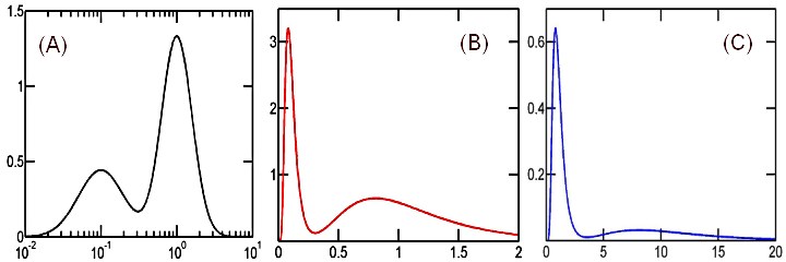
The following Figure shows a sample distribution in terms of pdf's for the random variables X, log(X) and 1/X, each plotted using its native horizontal-axis scale.
|
| |
Figure 1. Different graphs for the same probability distribution, represented by
the probability density functions for random variables log(X), X and 1/X,
each plotted using its respective native scale as the horizontal axis
A distribution has been constructed as a mixture of (a) log10-normal distribution with log-scale mean of -1 and standard deviation of 0.3 and (b) log10-normal distribution with log-scale mean of 0 and standard deviation of 0.2. The two components were mixed in proportion of 1/3 and 2/3, respectively. The pdf's for log(X), X and 1/X - all corresponding to this same distribution - were plotted using logarithmic (A) , linear (B) and inverse (C) horizontal scale axes, respectively. Curves (B),(C) were computed from curve (A) using Eqs.(11,13). Since, by construction, the plain geometric area under curve (A) is 1, so are also the areas under the other two curves.
| |
Possible sources of confusion
Let us now limit our discussion to just two different random variables: X and log(X). We shall consider a single statistical distribution for X given by [1], which, through the elementary recipe
| | |

| (14) | |
defines also the distribution of log(X).
While the distribution is the same, the corresponding probability density functions ρllin and ρlog are different according to whether they are computed for the random variable X (linvar case) or for the random variable log(X) (logvar case). This is further complicated by the fact that both functions can be graphically displayed using either linear or logarithmic horizontal axis (linaxis or logaxis, respectively). The two things have nothing in common, all four cross-combinations are perfectly legitimate, as long as one knows exactly which is the chosen case. The possible confusion arises from the fact that the same term 'scale' is often applied to both the chosen random variable (X or log(X)) and the horizontal axis used to plot the functions (this latter aspect being just a mere display option which has nothing to do with probability theory).
In order to reduce the sources of confusion, however, it is recommendable to always represent linvar probability densities using graphs with linear axes and logvar probability densities using graphs with logarithmic axes. Only in these cases, in fact, can one apply the intuitive Riemann integration and avoid the less instinctive Lebesque integral with a non-linear measure.
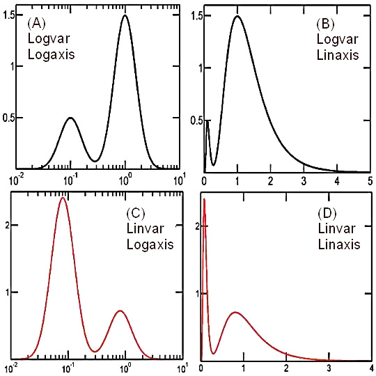
As an example, Figure 2. shows a probability distribution represented by means of probability density functions for the variables X and log(X), each expressed using both linear and logarithmic horizontal axes. Though the four graphs appear different from each other, they are all legitimate and they all represent exactly the same statistical distribution.
| |
Figure 2.
A probability distribution represented in four equivalent ways
A distribution has been constructed as a mixture of (a) log10-normal distribution with log-scale mean value of -1 and standard deviation of 0.2 and (b) log10-normal distribution with log-scale mean of 0 and standard deviation of 0.2. The two components were mixed in proportion of 1/4 and 3/4, respectively. The probability density functions for log(X) (logvar, ρ-log) and X (linvar, ρ-lin) corresponding to this distribution were plotted using two different horizontal axes: linear and logarithmic.
The four graphs obtained by combining the two alternatives are all equivalent and each of them is a legitimate representation of the same probability distribution. The privileged representations, however, are logvar/logaxis (A) and linvar/linaxis (D) since only in these cases the simple geometric areas under the two peaks, for example, have the correct ratio of 1:4.
| |
| |
References
- 1. Kolmogorov A.N., Foundations of the Theory of Probability,
Chelsea Pub Co., 2nd Edition 1960.
more >>
- 2. Feller W., An Introduction to Probability Theory and Its Applications,
Vol.1, John Wiley, 3rd Edition, 1968.
more >>
- 3. Gnedenko B.V., Theory of Probability, CRC 1998. 6th Edition.
more >>
- 4. Cramer H., Mathematical Methods of Statistics, Princeton University Press, Princeton, NJ, 1999.
more >>
- 5. Radhakrishna R., Linear Statistical Inference and Its Applications, John Wiley, 2nd Edition, 2002.
more >>
- 6. Weisstein E.W., The CRC Concise Encyclopedia of Mathematics, CRC Press 1998.
Online version.
more >>
- 7. Cramer H., Wold H., Some theorems on distribution functions, J.London Math.Soc. 11, 290, 1936.
See also.
- 8. Saks S., Theory of the Integral, Dover Publications, New York, 1964.
- 9. McWhirter J.G., Pike E.R., On the numerical inversion of the Laplace transform and similar Fredholm integral equations of the first kind, J.Phys.A:Math.Gen. 11,1729 (1978).
- 10. Provencher S.W., A constrained regularization method for inverting data represented by linear algebraic or integral equations, Computer Phys.Comm 27, 213 (1982).
- 11. Provencher S.W., CONTIN: A general purpose constrained regularization program for inverting noisy linear algebraic and integral equations, Computer Phys.Comm 27, 229 (1982).
- 12. Kroeker R.M., Henkelman R.M., Analysis of Biological NMR Relaxation Data with Continuous Distributions of Relaxation Times, J.Magn.Reson. 69,218 (1986).
- 13. Millhauser G.L., Carter A.A., Schneider D.J., Freed J.H., Oswald R.E., Rapid Singular Value Decomposition for Time-Domain Analysis of Magnetic Resonance Signals by Use of the Lanczos Algorithm, J.Magn.Reson. 82,150 (1989).
- 14. Jakes J.,Stepanek P., Positive exponential sum method of inverting Laplace transform applied to photon correlation spectroscopy, Czech.J.Phys. B40,972 (1990).
- 15. Lin Y.Y.,Ge N.H.,Hwang L.P., Multiexponential Analysis of Relaxation Decays Based on Linear Prediction and Singular-Value Decomposition, J.Magn.Reson. A105,65 (1993).
- 16. Jakes J., The peak constrained positive exponential sum method of inverting Laplace transform applied to correlation spectroscopy, Czech.J.Phys. B43,1 (1993).
- 17. Lupu M.,Todor D., A singular value decomposition based algorithm for multicomponent exponential fitting of NMR relaxation signals, Chemometrics and Intelligent Lab.Systems 29,11 (1995).
- 18. Borgia G.C., Brown R.J.S., Fantazzini P., Uniform Penalty Inversion of Multiexponential Decay Data, J.Magn.Reson. 132,65 (1998).
- 19. Borgia G.C., Brown R.J.S., Fantazzini P., Uniform Penalty Inversion of Multiexponential Decay Data II. Data Spacing, T2 Data, Systematic Data Errors, and Diagnostics, J.Magn.Reson. 147,273 (2000).
- 20. Borgia G.C., Brown R.J.S., Fantazzini P., Examples of marginal resolution of NMR relaxation peaks using UPEN and diagnostics, Magn.Reson.Imaging 19,473 (2001).
- 21. R.Lamanna, Visualization of Relaxation Properties through the Inversion of Exponential Decays, XXXIV National Congress on Magnetic Resonance, GIDRM, 2004.
Note added January 1, 2007: An introduction to the topics discussed in this article can be found also in
- 22. Capinski M., Kopp P.E., Measure, Integral and Probability, Springer Verlag 2004.
- 23. Suppes P., Zanotti M., Foundations of Probability with Applications, Cambridge University Press 2003.
|
|